


Vincent Selhorst-Jones
Systems of Linear Inequalities
Slide Duration:Table of Contents
Section 1: Introduction
Introduction to Precalculus
10m 3s
- Intro0:00
- Title of the Course0:06
- Different Names for the Course0:07
- Precalculus0:12
- Math Analysis0:14
- Trigonometry0:16
- Algebra III0:20
- Geometry II0:24
- College Algebra0:30
- Same Concepts0:36
- How do the Lessons Work?0:54
- Introducing Concepts0:56
- Apply Concepts1:04
- Go through Examples1:25
- Who is this Course For?1:38
- Those Who Need eExtra Help with Class Work1:52
- Those Working on Material but not in Formal Class at School1:54
- Those Who Want a Refresher2:00
- Try to Watch the Whole Lesson2:20
- Understanding is So Important3:56
- What to Watch First5:26
- Lesson #2: Sets, Elements, and Numbers5:30
- Lesson #7: Idea of a Function5:33
- Lesson #6: Word Problems6:04
- What to Watch First, cont.6:46
- Lesson #2: Sets, Elements and Numbers6:56
- Lesson #3: Variables, Equations, and Algebra6:58
- Lesson #4: Coordinate Systems7:00
- Lesson #5: Midpoint, Distance, the Pythagorean Theorem and Slope7:02
- Lesson #6: Word Problems7:10
- Lesson #7: Idea of a Function7:12
- Lesson #8: Graphs7:14
- Graphing Calculator Appendix7:40
- What to Watch Last8:46
- Let's get Started!9:48
Sets, Elements, & Numbers
45m 11s
- Intro0:00
- Introduction0:05
- Sets and Elements1:19
- Set1:20
- Element1:23
- Name a Set2:20
- Order The Elements Appear In Has No Effect on the Set2:55
- Describing/ Defining Sets3:28
- Directly Say All the Elements3:36
- Clearly Describing All the Members of the Set3:55
- Describing the Quality (or Qualities) Each member Of the Set Has In Common4:32
- Symbols: 'Element of' and 'Subset of'6:01
- Symbol is ∈6:03
- Subset Symbol is ⊂6:35
- Empty Set8:07
- Symbol is ∅8:20
- Since It's Empty, It is a Subset of All Sets8:44
- Union and Intersection9:54
- Union Symbol is ∪10:08
- Intersection Symbol is ∩10:18
- Sets Can Be Weird Stuff12:26
- Can Have Elements in a Set12:50
- We Can Have Infinite Sets13:09
- Example13:22
- Consider a Set Where We Take a Word and Then Repeat It An Ever Increasing Number of Times14:08
- This Set Has Infinitely Many Distinct Elements14:40
- Numbers as Sets16:03
- Natural Numbers ℕ16:16
- Including 0 and the Negatives ℤ18:13
- Rational Numbers ℚ19:27
- Can Express Rational Numbers with Decimal Expansions22:05
- Irrational Numbers23:37
- Real Numbers ℝ: Put the Rational and Irrational Numbers Together25:15
- Interval Notation and the Real Numbers26:45
- Include the End Numbers27:06
- Exclude the End Numbers27:33
- Example28:28
- Interval Notation: Infinity29:09
- Use -∞ or ∞ to Show an Interval Going on Forever in One Direction or the Other29:14
- Always Use Parentheses29:50
- Examples30:27
- Example 131:23
- Example 235:26
- Example 338:02
- Example 442:21
Variables, Equations, & Algebra
35m 31s
- Intro0:00
- What is a Variable?0:05
- A Variable is a Placeholder for a Number0:11
- Affects the Output of a Function or a Dependent Variable0:24
- Naming Variables1:51
- Useful to Use Symbols2:21
- What is a Constant?4:14
- A Constant is a Fixed, Unchanging Number4:28
- We Might Refer to a Symbol Representing a Number as a Constant4:51
- What is a Coefficient?5:33
- A Coefficient is a Multiplicative Factor on a Variable5:37
- Not All Coefficients are Constants5:51
- Expressions and Equations6:42
- An Expression is a String of Mathematical Symbols That Make Sense Used Together7:05
- An Equation is a Statement That Two Expression Have the Same Value8:20
- The Idea of Algebra8:51
- Equality8:59
- If Two Things Are the Same *Equal), Then We Can Do the Exact Same Operation to Both and the Results Will Be the Same9:41
- Always Do The Exact Same Thing to Both Sides12:22
- Solving Equations13:23
- When You Are Asked to Solve an Equation, You Are Being Asked to Solve for Something13:33
- Look For What Values Makes the Equation True13:38
- Isolate the Variable by Doing Algebra14:37
- Order of Operations16:02
- Why Certain Operations are Grouped17:01
- When You Don't Have to Worry About Order17:39
- Distributive Property18:15
- It Allows Multiplication to Act Over Addition in Parentheses18:23
- We Can Use the Distributive Property in Reverse to Combine Like Terms19:05
- Substitution20:03
- Use Information From One Equation in Another Equation20:07
- Put Your Substitution in Parentheses20:44
- Example 123:17
- Example 225:49
- Example 328:11
- Example 430:02
Coordinate Systems
35m 2s
- Intro0:00
- Inherent Order in ℝ0:05
- Real Numbers Come with an Inherent Order0:11
- Positive Numbers0:21
- Negative Numbers0:58
- 'Less Than' and 'Greater Than'2:04
- Tip To Help You Remember the Signs2:56
- Inequality4:06
- Less Than or Equal and Greater Than or Equal4:51
- One Dimension: The Number Line5:36
- Graphically Represent ℝ on a Number Line5:43
- Note on Infinities5:57
- With the Number Line, We Can Directly See the Order We Put on ℝ6:35
- Ordered Pairs7:22
- Example7:34
- Allows Us to Talk About Two Numbers at the Same Time9:41
- Ordered Pairs of Real Numbers Cannot be Put Into an Order Like we Did with ℝ10:41
- Two Dimensions: The Plane13:13
- We Can Represent Ordered Pairs with the Plane13:24
- Intersection is known as the Origin14:31
- Plotting the Point14:32
- Plane = Coordinate Plane = Cartesian Plane = ℝ²17:46
- The Plane and Quadrants18:50
- Quadrant I19:04
- Quadrant II19:21
- Quadrant III20:04
- Quadrant IV20:20
- Three Dimensions: Space21:02
- Create Ordered Triplets21:09
- Visually Represent This21:19
- Three-Dimension = Space = ℝ³21:47
- Higher Dimensions22:24
- If We Have n Dimensions, We Call It n-Dimensional Space or ℝ to the nth Power22:31
- We Can Represent Places In This n-Dimensional Space As Ordered Groupings of n Numbers22:41
- Hard to Visualize Higher Dimensional Spaces23:18
- Example 125:07
- Example 226:10
- Example 328:58
- Example 431:05
Midpoints, Distance, the Pythagorean Theorem, & Slope
48m 43s
- Intro0:00
- Introduction0:07
- Midpoint: One Dimension2:09
- Example of Something More Complex2:31
- Use the Idea of a Middle3:28
- Find the Midpoint of Arbitrary Values a and b4:17
- How They're Equivalent5:05
- Official Midpoint Formula5:46
- Midpoint: Two Dimensions6:19
- The Midpoint Must Occur at the Horizontal Middle and the Vertical Middle6:38
- Arbitrary Pair of Points Example7:25
- Distance: One Dimension9:26
- Absolute Value10:54
- Idea of Forcing Positive11:06
- Distance: One Dimension, Formula11:47
- Distance Between Arbitrary a and b11:48
- Absolute Value Helps When the Distance is Negative12:41
- Distance Formula12:58
- The Pythagorean Theorem13:24
- a²+b²=c²13:50
- Distance: Two Dimensions14:59
- Break Into Horizontal and Vertical Parts and then Use the Pythagorean Theorem15:16
- Distance Between Arbitrary Points (x₁,y₁) and (x₂,y₂)16:21
- Slope19:30
- Slope is the Rate of Change19:41
- m = rise over run21:27
- Slope Between Arbitrary Points (x₁,y₁) and (x₂,y₂)22:31
- Interpreting Slope24:12
- Positive Slope and Negative Slope25:40
- m=1, m=0, m=-126:48
- Example 128:25
- Example 231:42
- Example 336:40
- Example 442:48
Word Problems
56m 31s
- Intro0:00
- Introduction0:05
- What is a Word Problem?0:45
- Describes Any Problem That Primarily Gets Its Ideas Across With Words Instead of Math Symbols0:48
- Requires Us to Think1:32
- Why Are They So Hard?2:11
- Reason 1: No Simple Formula to Solve Them2:16
- Reason 2: Harder to Teach Word Problems2:47
- You Can Learn How to Do Them!3:51
- Grades7:57
- 'But I'm Never Going to Use This In Real Life'9:46
- Solving Word Problems12:58
- First: Understand the Problem13:37
- Second: What Are You Looking For?14:33
- Third: Set Up Relationships16:21
- Fourth: Solve It!17:48
- Summary of Method19:04
- Examples on Things Other Than Math20:21
- Math-Specific Method: What You Need Now25:30
- Understand What the Problem is Talking About25:37
- Set Up and Name Any Variables You Need to Know25:56
- Set Up Equations Connecting Those Variables to the Information in the Problem Statement26:02
- Use the Equations to Solve for an Answer26:14
- Tip26:58
- Draw Pictures27:22
- Breaking Into Pieces28:28
- Try Out Hypothetical Numbers29:52
- Student Logic31:27
- Jump In!32:40
- Example 134:03
- Example 239:15
- Example 344:22
- Example 450:24
Section 2: Functions
Idea of a Function
39m 54s
- Intro0:00
- Introduction0:04
- What is a Function?1:06
- A Visual Example and Non-Example1:30
- Function Notation3:47
- f(x)4:05
- Express What Sets the Function Acts On5:45
- Metaphors for a Function6:17
- Transformation6:28
- Map7:17
- Machine8:56
- Same Input Always Gives Same Output10:01
- If We Put the Same Input Into a Function, It Will Always Produce the Same Output10:11
- Example of Something That is Not a Function11:10
- A Non-Numerical Example12:10
- The Functions We Will Use15:05
- Unless Told Otherwise, We Will Assume Every Function Takes in Real Numbers and Outputs Real Numbers15:11
- Usually Told the Rule of a Given Function15:27
- How To Use a Function16:18
- Apply the Rule to Whatever Our Input Value Is16:28
- Make Sure to Wrap Your Substitutions in Parentheses17:09
- Functions and Tables17:36
- Table of Values, Sometimes Called a T-Table17:46
- Example17:56
- Domain: What Goes In18:55
- The Domain is the Set of all Inputs That the Function Can Accept18:56
- Example19:40
- Range: What Comes Out21:27
- The Range is the Set of All Possible Outputs a Function Can Assign21:34
- Example21:49
- Another Example Would Be Our Initial Function From Earlier in This Lesson22:29
- Example 123:45
- Example 225:22
- Example 327:27
- Example 429:23
- Example 533:33
Graphs
58m 26s
- Intro0:00
- Introduction0:04
- How to Interpret Graphs1:17
- Input / Independent Variable1:47
- Output / Dependent Variable2:00
- Graph as Input ⇒ Output2:23
- One Way to Think of a Graph: See What Happened to Various Inputs2:25
- Example2:47
- Graph as Location of Solution4:20
- A Way to See Solutions4:36
- Example5:20
- Which Way Should We Interpret?7:13
- Easiest to Think In Terms of How Inputs Are Mapped to Outputs7:20
- Sometimes It's Easier to Think In Terms of Solutions8:39
- Pay Attention to Axes9:50
- Axes Tell Where the Graph Is and What Scale It Has10:09
- Often, The Axes Will Be Square10:14
- Example12:06
- Arrows or No Arrows?16:07
- Will Not Use Arrows at the End of Our Graphs17:13
- Graph Stops Because It Hits the Edge of the Graphing Axes, Not Because the Function Stops17:18
- How to Graph19:47
- Plot Points20:07
- Connect with Curves21:09
- If You Connect with Straight Lines21:44
- Graphs of Functions are Smooth22:21
- More Points ⇒ More Accurate23:38
- Vertical Line Test27:44
- If a Vertical Line Could Intersect More Than One Point On a Graph, It Can Not Be the Graph of a Function28:41
- Every Point on a Graph Tells Us Where the x-Value Below is Mapped30:07
- Domain in Graphs31:37
- The Domain is the Set of All Inputs That a Function Can Accept31:44
- Be Aware That Our Function Probably Continues Past the Edge of Our 'Viewing Window'33:19
- Range in Graphs33:53
- Graphing Calculators: Check the Appendix!36:55
- Example 138:37
- Example 245:19
- Example 350:41
- Example 453:28
- Example 555:50
Properties of Functions
48m 49s
- Intro0:00
- Introduction0:05
- Increasing Decreasing Constant0:43
- Looking at a Specific Graph1:15
- Increasing Interval2:39
- Constant Function4:15
- Decreasing Interval5:10
- Find Intervals by Looking at the Graph5:32
- Intervals Show x-values; Write in Parentheses6:39
- Maximum and Minimums8:48
- Relative (Local) Max/Min10:20
- Formal Definition of Relative Maximum12:44
- Formal Definition of Relative Minimum13:05
- Max/Min, More Terms14:18
- Definition of Extrema15:01
- Average Rate of Change16:11
- Drawing a Line for the Average Rate16:48
- Using the Slope of the Secant Line17:36
- Slope in Function Notation18:45
- Zeros/Roots/x-intercepts19:45
- What Zeros in a Function Mean20:25
- Even Functions22:30
- Odd Functions24:36
- Even/Odd Functions and Graphs26:28
- Example of an Even Function27:12
- Example of an Odd Function28:03
- Example 129:35
- Example 233:07
- Example 340:32
- Example 442:34
Function Petting Zoo
29m 20s
- Intro0:00
- Introduction0:04
- Don't Forget that Axes Matter!1:44
- The Constant Function2:40
- The Identity Function3:44
- The Square Function4:40
- The Cube Function5:44
- The Square Root Function6:51
- The Reciprocal Function8:11
- The Absolute Value Function10:19
- The Trigonometric Functions11:56
- f(x)=sin(x)12:12
- f(x)=cos(x)12:24
- Alternate Axes12:40
- The Exponential and Logarithmic Functions13:35
- Exponential Functions13:44
- Logarithmic Functions14:24
- Alternating Axes15:17
- Transformations and Compositions16:08
- Example 117:52
- Example 218:33
- Example 320:24
- Example 426:07
Transformation of Functions
48m 35s
- Intro0:00
- Introduction0:04
- Vertical Shift1:12
- Graphical Example1:21
- A Further Explanation2:16
- Vertical Stretch/Shrink3:34
- Graph Shrinks3:46
- Graph Stretches3:51
- A Further Explanation5:07
- Horizontal Shift6:49
- Moving the Graph to the Right7:28
- Moving the Graph to the Left8:12
- A Further Explanation8:19
- Understanding Movement on the x-axis8:38
- Horizontal Stretch/Shrink12:59
- Shrinking the Graph13:40
- Stretching the Graph13:48
- A Further Explanation13:55
- Understanding Stretches from the x-axis14:12
- Vertical Flip (aka Mirror)16:55
- Example Graph17:07
- Multiplying the Vertical Component by -117:18
- Horizontal Flip (aka Mirror)18:43
- Example Graph19:01
- Multiplying the Horizontal Component by -119:54
- Summary of Transformations22:11
- Stacking Transformations24:46
- Order Matters25:20
- Transformation Example25:52
- Example 129:21
- Example 234:44
- Example 338:10
- Example 443:46
Composite Functions
33m 24s
- Intro0:00
- Introduction0:04
- Arithmetic Combinations0:40
- Basic Operations1:20
- Definition of the Four Arithmetic Combinations1:40
- Composite Functions2:53
- The Function as a Machine3:32
- Function Compositions as Multiple Machines3:59
- Notation for Composite Functions4:46
- Two Formats6:02
- Another Visual Interpretation7:17
- How to Use Composite Functions8:21
- Example of on Function acting on Another9:17
- Example 111:03
- Example 215:27
- Example 321:11
- Example 427:06
Piecewise Functions
51m 42s
- Intro0:00
- Introduction0:04
- Analogies to a Piecewise Function1:16
- Different Potatoes1:41
- Factory Production2:27
- Notations for Piecewise Functions3:39
- Notation Examples from Analogies6:11
- Example of a Piecewise (with Table)7:24
- Example of a Non-Numerical Piecewise11:35
- Graphing Piecewise Functions14:15
- Graphing Piecewise Functions, Example16:26
- Continuous Functions16:57
- Statements of Continuity19:30
- Example of Continuous and Non-Continuous Graphs20:05
- Interesting Functions: the Step Function22:00
- Notation for the Step Function22:40
- How the Step Function Works22:56
- Graph of the Step Function25:30
- Example 126:22
- Example 228:49
- Example 336:50
- Example 446:11
Inverse Functions
49m 37s
- Intro0:00
- Introduction0:04
- Analogy by picture1:10
- How to Denote the inverse1:40
- What Comes out of the Inverse1:52
- Requirement for Reversing2:02
- The Basketball Factory2:12
- The Importance of Information2:45
- One-to-One4:04
- Requirement for Reversibility4:21
- When a Function has an Inverse4:43
- One-to-One5:13
- Not One-to-One5:50
- Not a Function6:19
- Horizontal Line Test7:01
- How to the test Works7:12
- One-to-One8:12
- Not One-to-One8:45
- Definition: Inverse Function9:12
- Formal Definition9:21
- Caution to Students10:02
- Domain and Range11:12
- Finding the Range of the Function Inverse11:56
- Finding the Domain of the Function Inverse12:11
- Inverse of an Inverse13:09
- Its just x!13:26
- Proof14:03
- Graphical Interpretation17:07
- Horizontal Line Test17:20
- Graph of the Inverse18:04
- Swapping Inputs and Outputs to Draw Inverses19:02
- How to Find the Inverse21:03
- What We Are Looking For21:21
- Reversing the Function21:38
- A Method to Find Inverses22:33
- Check Function is One-to-One23:04
- Swap f(x) for y23:25
- Interchange x and y23:41
- Solve for y24:12
- Replace y with the inverse24:40
- Some Comments25:01
- Keeping Step 2 and 3 Straight25:44
- Switching to Inverse26:12
- Checking Inverses28:52
- How to Check an Inverse29:06
- Quick Example of How to Check29:56
- Example 131:48
- Example 234:56
- Example 339:29
- Example 446:19
Variation Direct and Inverse
28m 49s
- Intro0:00
- Introduction0:06
- Direct Variation1:14
- Same Direction1:21
- Common Example: Groceries1:56
- Different Ways to Say that Two Things Vary Directly2:28
- Basic Equation for Direct Variation2:55
- Inverse Variation3:40
- Opposite Direction3:50
- Common Example: Gravity4:53
- Different Ways to Say that Two Things Vary Indirectly5:48
- Basic Equation for Indirect Variation6:33
- Joint Variation7:27
- Equation for Joint Variation7:53
- Explanation of the Constant8:48
- Combined Variation9:35
- Gas Law as a Combination9:44
- Single Constant10:33
- Example 110:49
- Example 213:34
- Example 315:39
- Example 419:48
Section 3: Polynomials
Intro to Polynomials
38m 41s
- Intro0:00
- Introduction0:04
- Definition of a Polynomial1:04
- Starting Integer2:06
- Structure of a Polynomial2:49
- The a Constants3:34
- Polynomial Function5:13
- Polynomial Equation5:23
- Polynomials with Different Variables5:36
- Degree6:23
- Informal Definition6:31
- Find the Largest Exponent Variable6:44
- Quick Examples7:36
- Special Names for Polynomials8:59
- Based on the Degree9:23
- Based on the Number of Terms10:12
- Distributive Property (aka 'FOIL')11:37
- Basic Distributive Property12:21
- Distributing Two Binomials12:55
- Longer Parentheses15:12
- Reverse: Factoring17:26
- Long-Term Behavior of Polynomials17:48
- Examples18:13
- Controlling Term--Term with the Largest Exponent19:33
- Positive and Negative Coefficients on the Controlling Term20:21
- Leading Coefficient Test22:07
- Even Degree, Positive Coefficient22:13
- Even Degree, Negative Coefficient22:39
- Odd Degree, Positive Coefficient23:09
- Odd Degree, Negative Coefficient23:27
- Example 125:11
- Example 227:16
- Example 331:16
- Example 434:41
Roots (Zeros) of Polynomials
41m 7s
- Intro0:00
- Introduction0:05
- Roots in Graphs1:17
- The x-intercepts1:33
- How to Remember What 'Roots' Are1:50
- Naïve Attempts2:31
- Isolating Variables2:45
- Failures of Isolating Variables3:30
- Missing Solutions4:59
- Factoring: How to Find Roots6:28
- How Factoring Works6:36
- Why Factoring Works7:20
- Steps to Finding Polynomial Roots9:21
- Factoring: How to Find Roots CAUTION10:08
- Factoring is Not Easy11:32
- Factoring Quadratics13:08
- Quadratic Trinomials13:21
- Form of Factored Binomials13:38
- Factoring Examples14:40
- Factoring Quadratics, Check Your Work16:58
- Factoring Higher Degree Polynomials18:19
- Factoring a Cubic18:32
- Factoring a Quadratic19:04
- Factoring: Roots Imply Factors19:54
- Where a Root is, A Factor Is20:01
- How to Use Known Roots to Make Factoring Easier20:35
- Not all Polynomials Can be Factored22:30
- Irreducible Polynomials23:27
- Complex Numbers Help23:55
- Max Number of Roots/Factors24:57
- Limit to Number of Roots Equal to the Degree25:18
- Why there is a Limit25:25
- Max Number of Peaks/Valleys26:39
- Shape Information from Degree26:46
- Example Graph26:54
- Max, But Not Required28:00
- Example 128:37
- Example 231:21
- Example 336:12
- Example 438:40
Completing the Square and the Quadratic Formula
39m 43s
- Intro0:00
- Introduction0:05
- Square Roots and Equations0:51
- Taking the Square Root to Find the Value of x0:55
- Getting the Positive and Negative Answers1:05
- Completing the Square: Motivation2:04
- Polynomials that are Easy to Solve2:20
- Making Complex Polynomials Easy to Solve3:03
- Steps to Completing the Square4:30
- Completing the Square: Method7:22
- Move C over7:35
- Divide by A7:44
- Find r7:59
- Add to Both Sides to Complete the Square8:49
- Solving Quadratics with Ease9:56
- The Quadratic Formula11:38
- Derivation11:43
- Final Form12:23
- Follow Format to Use Formula13:38
- How Many Roots?14:53
- The Discriminant15:47
- What the Discriminant Tells Us: How Many Roots15:58
- How the Discriminant Works16:30
- Example 1: Complete the Square18:24
- Example 2: Solve the Quadratic22:00
- Example 3: Solve for Zeroes25:28
- Example 4: Using the Quadratic Formula30:52
Properties of Quadratic Functions
45m 34s
- Intro0:00
- Introduction0:05
- Parabolas0:35
- Examples of Different Parabolas1:06
- Axis of Symmetry and Vertex1:28
- Drawing an Axis of Symmetry1:51
- Placing the Vertex2:28
- Looking at the Axis of Symmetry and Vertex for other Parabolas3:09
- Transformations4:18
- Reviewing Transformation Rules6:28
- Note the Different Horizontal Shift Form7:45
- An Alternate Form to Quadratics8:54
- The Constants: k, h, a9:05
- Transformations Formed10:01
- Analyzing Different Parabolas10:10
- Switching Forms by Completing the Square11:43
- Vertex of a Parabola16:30
- Vertex at (h, k)16:47
- Vertex in Terms of a, b, and c Coefficients17:28
- Minimum/Maximum at Vertex18:19
- When a is Positive18:25
- When a is Negative18:52
- Axis of Symmetry19:54
- Incredibly Minor Note on Grammar20:52
- Example 121:48
- Example 226:35
- Example 328:55
- Example 431:40
Intermediate Value Theorem and Polynomial Division
46m 8s
- Intro0:00
- Introduction0:05
- Reminder: Roots Imply Factors1:32
- The Intermediate Value Theorem3:41
- The Basis: U between a and b4:11
- U is on the Function4:52
- Intermediate Value Theorem, Proof Sketch5:51
- If Not True, the Graph Would Have to Jump5:58
- But Graph is Defined as Continuous6:43
- Finding Roots with the Intermediate Value Theorem7:01
- Picking a and b to be of Different Signs7:10
- Must Be at Least One Root7:46
- Dividing a Polynomial8:16
- Using Roots and Division to Factor8:38
- Long Division Refresher9:08
- The Division Algorithm12:18
- How It Works to Divide Polynomials12:37
- The Parts of the Equation13:24
- Rewriting the Equation14:47
- Polynomial Long Division16:20
- Polynomial Long Division In Action16:29
- One Step at a Time20:51
- Synthetic Division22:46
- Setup23:11
- Synthetic Division, Example24:44
- Which Method Should We Use26:39
- Advantages of Synthetic Method26:49
- Advantages of Long Division27:13
- Example 129:24
- Example 231:27
- Example 336:22
- Example 440:55
Complex Numbers
45m 36s
- Intro0:00
- Introduction0:04
- A Wacky Idea1:02
- The Definition of the Imaginary Number1:22
- How it Helps Solve Equations2:20
- Square Roots and Imaginary Numbers3:15
- Complex Numbers5:00
- Real Part and Imaginary Part5:20
- When Two Complex Numbers are Equal6:10
- Addition and Subtraction6:40
- Deal with Real and Imaginary Parts Separately7:36
- Two Quick Examples7:54
- Multiplication9:07
- FOIL Expansion9:14
- Note What Happens to the Square of the Imaginary Number9:41
- Two Quick Examples10:22
- Division11:27
- Complex Conjugates13:37
- Getting Rid of i14:08
- How to Denote the Conjugate14:48
- Division through Complex Conjugates16:11
- Multiply by the Conjugate of the Denominator16:28
- Example17:46
- Factoring So-Called 'Irreducible' Quadratics19:24
- Revisiting the Quadratic Formula20:12
- Conjugate Pairs20:37
- But Are the Complex Numbers 'Real'?21:27
- What Makes a Number Legitimate25:38
- Where Complex Numbers are Used27:20
- Still, We Won't See Much of C29:05
- Example 130:30
- Example 233:15
- Example 338:12
- Example 442:07
Fundamental Theorem of Algebra
19m 9s
- Intro0:00
- Introduction0:05
- Idea: Hidden Roots1:16
- Roots in Complex Form1:42
- All Polynomials Have Roots2:08
- Fundamental Theorem of Algebra2:21
- Where Are All the Imaginary Roots, Then?3:17
- All Roots are Complex3:45
- Real Numbers are a Subset of Complex Numbers3:59
- The n Roots Theorem5:01
- For Any Polynomial, Its Degree is Equal to the Number of Roots5:11
- Equivalent Statement5:24
- Comments: Multiplicity6:29
- Non-Distinct Roots6:59
- Denoting Multiplicity7:20
- Comments: Complex Numbers Necessary7:41
- Comments: Complex Coefficients Allowed8:55
- Comments: Existence Theorem9:59
- Proof Sketch of n Roots Theorem10:45
- First Root11:36
- Second Root13:23
- Continuation to Find all Roots16:00
Section 4: Rational Functions
Rational Functions and Vertical Asymptotes
33m 22s
- Intro0:00
- Introduction0:05
- Definition of a Rational Function1:20
- Examples of Rational Functions2:30
- Why They are Called 'Rational'2:47
- Domain of a Rational Function3:15
- Undefined at Denominator Zeros3:25
- Otherwise all Reals4:16
- Investigating a Fundamental Function4:50
- The Domain of the Function5:04
- What Occurs at the Zeroes of the Denominator5:20
- Idea of a Vertical Asymptote6:23
- What's Going On?6:58
- Approaching x=0 from the left7:32
- Approaching x=0 from the right8:34
- Dividing by Very Small Numbers Results in Very Large Numbers9:31
- Definition of a Vertical Asymptote10:05
- Vertical Asymptotes and Graphs11:15
- Drawing Asymptotes by Using a Dashed Line11:27
- The Graph Can Never Touch Its Undefined Point12:00
- Not All Zeros Give Asymptotes13:02
- Special Cases: When Numerator and Denominator Go to Zero at the Same Time14:58
- Cancel out Common Factors15:49
- How to Find Vertical Asymptotes16:10
- Figure out What Values Are Not in the Domain of x16:24
- Determine if the Numerator and Denominator Share Common Factors and Cancel16:45
- Find Denominator Roots17:33
- Note if Asymptote Approaches Negative or Positive Infinity18:06
- Example 118:57
- Example 221:26
- Example 323:04
- Example 430:01
Horizontal Asymptotes
34m 16s
- Intro0:00
- Introduction0:05
- Investigating a Fundamental Function0:53
- What Happens as x Grows Large1:00
- Different View1:12
- Idea of a Horizontal Asymptote1:36
- What's Going On?2:24
- What Happens as x Grows to a Large Negative Number2:49
- What Happens as x Grows to a Large Number3:30
- Dividing by Very Large Numbers Results in Very Small Numbers3:52
- Example Function4:41
- Definition of a Vertical Asymptote8:09
- Expanding the Idea9:03
- What's Going On?9:48
- What Happens to the Function in the Long Run?9:51
- Rewriting the Function10:13
- Definition of a Slant Asymptote12:09
- Symbolical Definition12:30
- Informal Definition12:45
- Beyond Slant Asymptotes13:03
- Not Going Beyond Slant Asymptotes14:39
- Horizontal/Slant Asymptotes and Graphs15:43
- How to Find Horizontal and Slant Asymptotes16:52
- How to Find Horizontal Asymptotes17:12
- Expand the Given Polynomials17:18
- Compare the Degrees of the Numerator and Denominator17:40
- How to Find Slant Asymptotes20:05
- Slant Asymptotes Exist When n+m=120:08
- Use Polynomial Division20:24
- Example 124:32
- Example 225:53
- Example 326:55
- Example 429:22
Graphing Asymptotes in a Nutshell
49m 7s
- Intro0:00
- Introduction0:05
- A Process for Graphing1:22
- 1. Factor Numerator and Denominator1:50
- 2. Find Domain2:53
- 3. Simplifying the Function3:59
- 4. Find Vertical Asymptotes4:59
- 5. Find Horizontal/Slant Asymptotes5:24
- 6. Find Intercepts7:35
- 7. Draw Graph (Find Points as Necessary)9:21
- Draw Graph Example11:21
- Vertical Asymptote11:41
- Horizontal Asymptote11:50
- Other Graphing12:16
- Test Intervals15:08
- Example 117:57
- Example 223:01
- Example 329:02
- Example 433:37
Partial Fractions
44m 56s
- Intro0:00
- Introduction: Idea0:04
- Introduction: Prerequisites and Uses1:57
- Proper vs. Improper Polynomial Fractions3:11
- Possible Things in the Denominator4:38
- Linear Factors6:16
- Example of Linear Factors7:03
- Multiple Linear Factors7:48
- Irreducible Quadratic Factors8:25
- Example of Quadratic Factors9:26
- Multiple Quadratic Factors9:49
- Mixing Factor Types10:28
- Figuring Out the Numerator11:10
- How to Solve for the Constants11:30
- Quick Example11:40
- Example 114:29
- Example 218:35
- Example 320:33
- Example 428:51
Section 5: Exponential & Logarithmic Functions
Understanding Exponents
35m 17s
- Intro0:00
- Introduction0:05
- Fundamental Idea1:46
- Expanding the Idea2:28
- Multiplication of the Same Base2:40
- Exponents acting on Exponents3:45
- Different Bases with the Same Exponent4:31
- To the Zero5:35
- To the First5:45
- Fundamental Rule with the Zero Power6:35
- To the Negative7:45
- Any Number to a Negative Power8:14
- A Fraction to a Negative Power9:58
- Division with Exponential Terms10:41
- To the Fraction11:33
- Square Root11:58
- Any Root12:59
- Summary of Rules14:38
- To the Irrational17:21
- Example 120:34
- Example 223:42
- Example 327:44
- Example 431:44
- Example 533:15
Exponential Functions
47m 4s
- Intro0:00
- Introduction0:05
- Definition of an Exponential Function0:48
- Definition of the Base1:02
- Restrictions on the Base1:16
- Computing Exponential Functions2:29
- Harder Computations3:10
- When to Use a Calculator3:21
- Graphing Exponential Functions: a>16:02
- Three Examples6:13
- What to Notice on the Graph7:44
- A Story8:27
- Story Diagram9:15
- Increasing Exponentials11:29
- Story Morals14:40
- Application: Compound Interest15:15
- Compounding Year after Year16:01
- Function for Compounding Interest16:51
- A Special Number: e20:55
- Expression for e21:28
- Where e stabilizes21:55
- Application: Continuously Compounded Interest24:07
- Equation for Continuous Compounding24:22
- Exponential Decay 0<a<125:50
- Three Examples26:11
- Why they 'lose' value26:54
- Example 127:47
- Example 233:11
- Example 336:34
- Example 441:28
Introduction to Logarithms
40m 31s
- Intro0:00
- Introduction0:04
- Definition of a Logarithm, Base 20:51
- Log 2 Defined0:55
- Examples2:28
- Definition of a Logarithm, General3:23
- Examples of Logarithms5:15
- Problems with Unusual Bases7:38
- Shorthand Notation: ln and log9:44
- base e as ln10:01
- base 10 as log10:34
- Calculating Logarithms11:01
- using a calculator11:34
- issues with other bases11:58
- Graphs of Logarithms13:21
- Three Examples13:29
- Slow Growth15:19
- Logarithms as Inverse of Exponentiation16:02
- Using Base 216:05
- General Case17:10
- Looking More Closely at Logarithm Graphs19:16
- The Domain of Logarithms20:41
- Thinking about Logs like Inverses21:08
- The Alternate24:00
- Example 125:59
- Example 230:03
- Example 332:49
- Example 437:34
Properties of Logarithms
42m 33s
- Intro0:00
- Introduction0:04
- Basic Properties1:12
- Inverse--log(exp)1:43
- A Key Idea2:44
- What We Get through Exponentiation3:18
- B Always Exists4:50
- Inverse--exp(log)5:53
- Logarithm of a Power7:44
- Logarithm of a Product10:07
- Logarithm of a Quotient13:48
- Caution! There Is No Rule for loga(M+N)16:12
- Summary of Properties17:42
- Change of Base--Motivation20:17
- No Calculator Button20:59
- A Specific Example21:45
- Simplifying23:45
- Change of Base--Formula24:14
- Example 125:47
- Example 229:08
- Example 331:14
- Example 434:13
Solving Exponential and Logarithmic Equations
34m 10s
- Intro0:00
- Introduction0:05
- One to One Property1:09
- Exponential1:26
- Logarithmic1:44
- Specific Considerations2:02
- One-to-One Property3:30
- Solving by One-to-One4:11
- Inverse Property6:09
- Solving by Inverses7:25
- Dealing with Equations7:50
- Example of Taking an Exponent or Logarithm of an Equation9:07
- A Useful Property11:57
- Bring Down Exponents12:01
- Try to Simplify13:20
- Extraneous Solutions13:45
- Example 116:37
- Example 219:39
- Example 321:37
- Example 426:45
- Example 529:37
Application of Exponential and Logarithmic Functions
48m 46s
- Intro0:00
- Introduction0:06
- Applications of Exponential Functions1:07
- A Secret!2:17
- Natural Exponential Growth Model3:07
- Figure out r3:34
- A Secret!--Why Does It Work?4:44
- e to the r Morphs4:57
- Example5:06
- Applications of Logarithmic Functions8:32
- Examples8:43
- What Logarithms are Useful For9:53
- Example 111:29
- Example 215:30
- Example 326:22
- Example 432:05
- Example 539:19
Section 6: Trigonometric Functions
Angles
39m 5s
- Intro0:00
- Degrees0:22
- Circle is 360 Degrees0:48
- Splitting a Circle1:13
- Radians2:08
- Circle is 2 Pi Radians2:31
- One Radian2:52
- Half-Circle and Right Angle4:00
- Converting Between Degrees and Radians6:24
- Formulas for Degrees and Radians6:52
- Coterminal, Complementary, Supplementary Angles7:23
- Coterminal Angles7:30
- Complementary Angles9:40
- Supplementary Angles10:08
- Example 1: Dividing a Circle10:38
- Example 2: Converting Between Degrees and Radians11:56
- Example 3: Quadrants and Coterminal Angles14:18
- Extra Example 1: Common Angle Conversions-1
- Extra Example 2: Quadrants and Coterminal Angles-2
Sine and Cosine Functions
43m 16s
- Intro0:00
- Sine and Cosine0:15
- Unit Circle0:22
- Coordinates on Unit Circle1:03
- Right Triangles1:52
- Adjacent, Opposite, Hypotenuse2:25
- Master Right Triangle Formula: SOHCAHTOA2:48
- Odd Functions, Even Functions4:40
- Example: Odd Function4:56
- Example: Even Function7:30
- Example 1: Sine and Cosine10:27
- Example 2: Graphing Sine and Cosine Functions14:39
- Example 3: Right Triangle21:40
- Example 4: Odd, Even, or Neither26:01
- Extra Example 1: Right Triangle-1
- Extra Example 2: Graphing Sine and Cosine Functions-2
Sine and Cosine Values of Special Angles
33m 5s
- Intro0:00
- 45-45-90 Triangle and 30-60-90 Triangle0:08
- 45-45-90 Triangle0:21
- 30-60-90 Triangle2:06
- Mnemonic: All Students Take Calculus (ASTC)5:21
- Using the Unit Circle5:59
- New Angles6:21
- Other Quadrants9:43
- Mnemonic: All Students Take Calculus10:13
- Example 1: Convert, Quadrant, Sine/Cosine13:11
- Example 2: Convert, Quadrant, Sine/Cosine16:48
- Example 3: All Angles and Quadrants20:21
- Extra Example 1: Convert, Quadrant, Sine/Cosine-1
- Extra Example 2: All Angles and Quadrants-2
Modified Sine Waves: Asin(Bx+C)+D and Acos(Bx+C)+D
52m 3s
- Intro0:00
- Amplitude and Period of a Sine Wave0:38
- Sine Wave Graph0:58
- Amplitude: Distance from Middle to Peak1:18
- Peak: Distance from Peak to Peak2:41
- Phase Shift and Vertical Shift4:13
- Phase Shift: Distance Shifted Horizontally4:16
- Vertical Shift: Distance Shifted Vertically6:48
- Example 1: Amplitude/Period/Phase and Vertical Shift8:04
- Example 2: Amplitude/Period/Phase and Vertical Shift17:39
- Example 3: Find Sine Wave Given Attributes25:23
- Extra Example 1: Amplitude/Period/Phase and Vertical Shift-1
- Extra Example 2: Find Cosine Wave Given Attributes-2
Tangent and Cotangent Functions
36m 4s
- Intro0:00
- Tangent and Cotangent Definitions0:21
- Tangent Definition0:25
- Cotangent Definition0:47
- Master Formula: SOHCAHTOA1:01
- Mnemonic1:16
- Tangent and Cotangent Values2:29
- Remember Common Values of Sine and Cosine2:46
- 90 Degrees Undefined4:36
- Slope and Menmonic: ASTC5:47
- Uses of Tangent5:54
- Example: Tangent of Angle is Slope6:09
- Sign of Tangent in Quadrants7:49
- Example 1: Graph Tangent and Cotangent Functions10:42
- Example 2: Tangent and Cotangent of Angles16:09
- Example 3: Odd, Even, or Neither18:56
- Extra Example 1: Tangent and Cotangent of Angles-1
- Extra Example 2: Tangent and Cotangent of Angles-2
Secant and Cosecant Functions
27m 18s
- Intro0:00
- Secant and Cosecant Definitions0:17
- Secant Definition0:18
- Cosecant Definition0:33
- Example 1: Graph Secant Function0:48
- Example 2: Values of Secant and Cosecant6:49
- Example 3: Odd, Even, or Neither12:49
- Extra Example 1: Graph of Cosecant Function-1
- Extra Example 2: Values of Secant and Cosecant-2
Inverse Trigonometric Functions
32m 58s
- Intro0:00
- Arcsine Function0:24
- Restrictions between -1 and 10:43
- Arcsine Notation1:26
- Arccosine Function3:07
- Restrictions between -1 and 13:36
- Cosine Notation3:53
- Arctangent Function4:30
- Between -Pi/2 and Pi/24:44
- Tangent Notation5:02
- Example 1: Domain/Range/Graph of Arcsine5:45
- Example 2: Arcsin/Arccos/Arctan Values10:46
- Example 3: Domain/Range/Graph of Arctangent17:14
- Extra Example 1: Domain/Range/Graph of Arccosine-1
- Extra Example 2: Arcsin/Arccos/Arctan Values-2
Computations of Inverse Trigonometric Functions
31m 8s
- Intro0:00
- Inverse Trigonometric Function Domains and Ranges0:31
- Arcsine0:41
- Arccosine1:14
- Arctangent1:41
- Example 1: Arcsines of Common Values2:44
- Example 2: Odd, Even, or Neither5:57
- Example 3: Arccosines of Common Values12:24
- Extra Example 1: Arctangents of Common Values-1
- Extra Example 2: Arcsin/Arccos/Arctan Values-2
Section 7: Trigonometric Identities
Pythagorean Identity
19m 11s
- Intro0:00
- Pythagorean Identity0:17
- Pythagorean Triangle0:27
- Pythagorean Identity0:45
- Example 1: Use Pythagorean Theorem to Prove Pythagorean Identity1:14
- Example 2: Find Angle Given Cosine and Quadrant4:18
- Example 3: Verify Trigonometric Identity8:00
- Extra Example 1: Use Pythagorean Identity to Prove Pythagorean Theorem-1
- Extra Example 2: Find Angle Given Cosine and Quadrant-2
Identity Tan(squared)x+1=Sec(squared)x
23m 16s
- Intro0:00
- Main Formulas0:19
- Companion to Pythagorean Identity0:27
- For Cotangents and Cosecants0:52
- How to Remember0:58
- Example 1: Prove the Identity1:40
- Example 2: Given Tan Find Sec3:42
- Example 3: Prove the Identity7:45
- Extra Example 1: Prove the Identity-1
- Extra Example 2: Given Sec Find Tan-2
Addition and Subtraction Formulas
52m 52s
- Intro0:00
- Addition and Subtraction Formulas0:09
- How to Remember0:48
- Cofunction Identities1:31
- How to Remember Graphically1:44
- Where to Use Cofunction Identities2:52
- Example 1: Derive the Formula for cos(A-B)3:08
- Example 2: Use Addition and Subtraction Formulas16:03
- Example 3: Use Addition and Subtraction Formulas to Prove Identity25:11
- Extra Example 1: Use cos(A-B) and Cofunction Identities-1
- Extra Example 2: Convert to Radians and use Formulas-2
Double Angle Formulas
29m 5s
- Intro0:00
- Main Formula0:07
- How to Remember from Addition Formula0:18
- Two Other Forms1:35
- Example 1: Find Sine and Cosine of Angle using Double Angle3:16
- Example 2: Prove Trigonometric Identity using Double Angle9:37
- Example 3: Use Addition and Subtraction Formulas12:38
- Extra Example 1: Find Sine and Cosine of Angle using Double Angle-1
- Extra Example 2: Prove Trigonometric Identity using Double Angle-2
Half-Angle Formulas
43m 55s
- Intro0:00
- Main Formulas0:09
- Confusing Part0:34
- Example 1: Find Sine and Cosine of Angle using Half-Angle0:54
- Example 2: Prove Trigonometric Identity using Half-Angle11:51
- Example 3: Prove the Half-Angle Formula for Tangents18:39
- Extra Example 1: Find Sine and Cosine of Angle using Half-Angle-1
- Extra Example 2: Prove Trigonometric Identity using Half-Angle-2
Section 8: Applications of Trigonometry
Trigonometry in Right Angles
25m 43s
- Intro0:00
- Master Formula for Right Angles0:11
- SOHCAHTOA0:15
- Only for Right Triangles1:26
- Example 1: Find All Angles in a Triangle2:19
- Example 2: Find Lengths of All Sides of Triangle7:39
- Example 3: Find All Angles in a Triangle11:00
- Extra Example 1: Find All Angles in a Triangle-1
- Extra Example 2: Find Lengths of All Sides of Triangle-2
Law of Sines
56m 40s
- Intro0:00
- Law of Sines Formula0:18
- SOHCAHTOA0:27
- Any Triangle0:59
- Graphical Representation1:25
- Solving Triangle Completely2:37
- When to Use Law of Sines2:55
- ASA, SAA, SSA, AAA2:59
- SAS, SSS for Law of Cosines7:11
- Example 1: How Many Triangles Satisfy Conditions, Solve Completely8:44
- Example 2: How Many Triangles Satisfy Conditions, Solve Completely15:30
- Example 3: How Many Triangles Satisfy Conditions, Solve Completely28:32
- Extra Example 1: How Many Triangles Satisfy Conditions, Solve Completely-1
- Extra Example 2: How Many Triangles Satisfy Conditions, Solve Completely-2
Law of Cosines
49m 5s
- Intro0:00
- Law of Cosines Formula0:23
- Graphical Representation0:34
- Relates Sides to Angles1:00
- Any Triangle1:20
- Generalization of Pythagorean Theorem1:32
- When to Use Law of Cosines2:26
- SAS, SSS2:30
- Heron's Formula4:49
- Semiperimeter S5:11
- Example 1: How Many Triangles Satisfy Conditions, Solve Completely5:53
- Example 2: How Many Triangles Satisfy Conditions, Solve Completely15:19
- Example 3: Find Area of a Triangle Given All Side Lengths26:33
- Extra Example 1: How Many Triangles Satisfy Conditions, Solve Completely-1
- Extra Example 2: Length of Third Side and Area of Triangle-2
Finding the Area of a Triangle
27m 37s
- Intro0:00
- Master Right Triangle Formula and Law of Cosines0:19
- SOHCAHTOA0:27
- Law of Cosines1:23
- Heron's Formula2:22
- Semiperimeter S2:37
- Example 1: Area of Triangle with Two Sides and One Angle3:12
- Example 2: Area of Triangle with Three Sides6:11
- Example 3: Area of Triangle with Three Sides, No Heron's Formula8:50
- Extra Example 1: Area of Triangle with Two Sides and One Angle-1
- Extra Example 2: Area of Triangle with Two Sides and One Angle-2
Word Problems and Applications of Trigonometry
34m 25s
- Intro0:00
- Formulas to Remember0:11
- SOHCAHTOA0:15
- Law of Sines0:55
- Law of Cosines1:48
- Heron's Formula2:46
- Example 1: Telephone Pole Height4:01
- Example 2: Bridge Length7:48
- Example 3: Area of Triangular Field14:20
- Extra Example 1: Kite Height-1
- Extra Example 2: Roads to a Town-2
Section 9: Systems of Equations and Inequalities
Systems of Linear Equations
55m 40s
- Intro0:00
- Introduction0:04
- Graphs as Location of 'True'1:49
- All Locations that Make the Function True2:25
- Understand the Relationship Between Solutions and the Graph3:43
- Systems as Graphs4:07
- Equations as Lines4:20
- Intersection Point5:19
- Three Possibilities for Solutions6:17
- Independent6:24
- Inconsistent6:36
- Dependent7:06
- Solving by Substitution8:37
- Solve for One Variable9:07
- Substitute into the Second Equation9:34
- Solve for Both Variables10:12
- What If a System is Inconsistent or Dependent?11:08
- No Solutions11:25
- Infinite Solutions12:30
- Solving by Elimination13:56
- Example14:22
- Determining the Number of Solutions16:30
- Why Elimination Makes Sense17:25
- Solving by Graphing Calculator19:59
- Systems with More than Two Variables23:22
- Example 125:49
- Example 230:22
- Example 334:11
- Example 438:55
- Example 546:01
- (Non-) Example 653:37
Systems of Linear Inequalities
1h 13s
- Intro0:00
- Introduction0:04
- Inequality Refresher-Solutions0:46
- Equation Solutions vs. Inequality Solutions1:02
- Essentially a Wide Variety of Answers1:35
- Refresher--Negative Multiplication Flips1:43
- Refresher--Negative Flips: Why?3:19
- Multiplication by a Negative3:43
- The Relationship Flips3:55
- Refresher--Stick to Basic Operations4:34
- Linear Equations in Two Variables6:50
- Graphing Linear Inequalities8:28
- Why It Includes a Whole Section8:43
- How to Show The Difference Between Strict and Not Strict Inequalities10:08
- Dashed Line--Not Solutions11:10
- Solid Line--Are Solutions11:24
- Test Points for Shading11:42
- Example of Using a Point12:41
- Drawing Shading from the Point13:14
- Graphing a System14:53
- Set of Solutions is the Overlap15:17
- Example15:22
- Solutions are Best Found Through Graphing18:05
- Linear Programming-Idea19:52
- Use a Linear Objective Function20:15
- Variables in Objective Function have Constraints21:24
- Linear Programming-Method22:09
- Rearrange Equations22:21
- Graph22:49
- Critical Solution is at the Vertex of the Overlap23:40
- Try Each Vertice24:35
- Example 124:58
- Example 228:57
- Example 333:48
- Example 443:10
Nonlinear Systems
41m 1s
- Intro0:00
- Introduction0:06
- Substitution1:12
- Example1:22
- Elimination3:46
- Example3:56
- Elimination is Less Useful for Nonlinear Systems4:56
- Graphing5:56
- Using a Graphing Calculator6:44
- Number of Solutions8:44
- Systems of Nonlinear Inequalities10:02
- Graph Each Inequality10:06
- Dashed and/or Solid10:18
- Shade Appropriately11:14
- Example 113:24
- Example 215:50
- Example 322:02
- Example 429:06
- Example 4, cont.33:40
Section 10: Vectors and Matrices
Vectors
1h 9m 31s
- Intro0:00
- Introduction0:10
- Magnitude of the Force0:22
- Direction of the Force0:48
- Vector0:52
- Idea of a Vector1:30
- How Vectors are Denoted2:00
- Component Form3:20
- Angle Brackets and Parentheses3:50
- Magnitude/Length4:26
- Denoting the Magnitude of a Vector5:16
- Direction/Angle7:52
- Always Draw a Picture8:50
- Component Form from Magnitude & Angle10:10
- Scaling by Scalars14:06
- Unit Vectors16:26
- Combining Vectors - Algebraically18:10
- Combining Vectors - Geometrically19:54
- Resultant Vector20:46
- Alternate Component Form: i, j21:16
- The Zero Vector23:18
- Properties of Vectors24:20
- No Multiplication (Between Vectors)28:30
- Dot Product29:40
- Motion in a Medium30:10
- Fish in an Aquarium Example31:38
- More Than Two Dimensions33:12
- More Than Two Dimensions - Magnitude34:18
- Example 135:26
- Example 238:10
- Example 345:48
- Example 450:40
- Example 4, cont.56:07
- Example 51:01:32
Dot Product & Cross Product
35m 20s
- Intro0:00
- Introduction0:08
- Dot Product - Definition0:42
- Dot Product Results in a Scalar, Not a Vector2:10
- Example in Two Dimensions2:34
- Angle and the Dot Product2:58
- The Dot Product of Two Vectors is Deeply Related to the Angle Between the Two Vectors2:59
- Proof of Dot Product Formula4:14
- Won't Directly Help Us Better Understand Vectors4:18
- Dot Product - Geometric Interpretation4:58
- We Can Interpret the Dot Product as a Measure of How Long and How Parallel Two Vectors Are7:26
- Dot Product - Perpendicular Vectors8:24
- If the Dot Product of Two Vectors is 0, We Know They are Perpendicular to Each Other8:54
- Cross Product - Definition11:08
- Cross Product Only Works in Three Dimensions11:09
- Cross Product - A Mnemonic12:16
- The Determinant of a 3 x 3 Matrix and Standard Unit Vectors12:17
- Cross Product - Geometric Interpretations14:30
- The Right-Hand Rule15:17
- Cross Product - Geometric Interpretations Cont.17:00
- Example 118:40
- Example 222:50
- Example 324:04
- Example 426:20
- Bonus Round29:18
- Proof: Dot Product Formula29:24
- Proof: Dot Product Formula, cont.30:38
Matrices
54m 7s
- Intro0:00
- Introduction0:08
- Definition of a Matrix3:02
- Size or Dimension3:58
- Square Matrix4:42
- Denoted by Capital Letters4:56
- When are Two Matrices Equal?5:04
- Examples of Matrices6:44
- Rows x Columns6:46
- Talking About Specific Entries7:48
- We Use Capitals to Denote a Matrix and Lower Case to Denotes Its Entries8:32
- Using Entries to Talk About Matrices10:08
- Scalar Multiplication11:26
- Scalar = Real Number11:34
- Example12:36
- Matrix Addition13:08
- Example14:22
- Matrix Multiplication15:00
- Example18:52
- Matrix Multiplication, cont.19:58
- Matrix Multiplication and Order (Size)25:26
- Make Sure Their Orders are Compatible25:27
- Matrix Multiplication is NOT Commutative28:20
- Example30:08
- Special Matrices - Zero Matrix (0)32:48
- Zero Matrix Has 0 for All of its Entries32:49
- Special Matrices - Identity Matrix (I)34:14
- Identity Matrix is a Square Matrix That Has 1 for All Its Entries on the Main Diagonal and 0 for All Other Entries34:15
- Example 136:16
- Example 240:00
- Example 344:54
- Example 450:08
Determinants & Inverses of Matrices
47m 12s
- Intro0:00
- Introduction0:06
- Not All Matrices Are Invertible1:30
- What Must a Matrix Have to Be Invertible?2:08
- Determinant2:32
- The Determinant is a Real Number Associated With a Square Matrix2:38
- If the Determinant of a Matrix is Nonzero, the Matrix is Invertible3:40
- Determinant of a 2 x 2 Matrix4:34
- Think in Terms of Diagonals5:12
- Minors and Cofactors - Minors6:24
- Example6:46
- Minors and Cofactors - Cofactors8:00
- Cofactor is Closely Based on the Minor8:01
- Alternating Sign Pattern9:04
- Determinant of Larger Matrices10:56
- Example13:00
- Alternative Method for 3x3 Matrices16:46
- Not Recommended16:48
- Inverse of a 2 x 2 Matrix19:02
- Inverse of Larger Matrices20:00
- Using Inverse Matrices21:06
- When Multiplied Together, They Create the Identity Matrix21:24
- Example 123:45
- Example 227:21
- Example 332:49
- Example 436:27
- Finding the Inverse of Larger Matrices41:59
- General Inverse Method - Step 143:25
- General Inverse Method - Step 243:27
- General Inverse Method - Step 2, cont.43:27
- General Inverse Method - Step 345:15
Using Matrices to Solve Systems of Linear Equations
58m 34s
- Intro0:00
- Introduction0:12
- Augmented Matrix1:44
- We Can Represent the Entire Linear System With an Augmented Matrix1:50
- Row Operations3:22
- Interchange the Locations of Two Rows3:50
- Multiply (or Divide) a Row by a Nonzero Number3:58
- Add (or Subtract) a Multiple of One Row to Another4:12
- Row Operations - Keep Notes!5:50
- Suggested Symbols7:08
- Gauss-Jordan Elimination - Idea8:04
- Gauss-Jordan Elimination - Idea, cont.9:16
- Reduced Row-Echelon Form9:18
- Gauss-Jordan Elimination - Method11:36
- Begin by Writing the System As An Augmented Matrix11:38
- Gauss-Jordan Elimination - Method, cont.13:48
- Cramer's Rule - 2 x 2 Matrices17:08
- Cramer's Rule - n x n Matrices19:24
- Solving with Inverse Matrices21:10
- Solving Inverse Matrices, cont.25:28
- The Mighty (Graphing) Calculator26:38
- Example 129:56
- Example 233:56
- Example 337:00
- Example 3, cont.45:04
- Example 451:28
Section 11: Alternate Ways to Graph
Parametric Equations
53m 33s
- Intro0:00
- Introduction0:06
- Definition1:10
- Plane Curve1:24
- The Key Idea2:00
- Graphing with Parametric Equations2:52
- Same Graph, Different Equations5:04
- How Is That Possible?5:36
- Same Graph, Different Equations, cont.5:42
- Here's Another to Consider7:56
- Same Plane Curve, But Still Different8:10
- A Metaphor for Parametric Equations9:36
- Think of Parametric Equations As a Way to Describe the Motion of An Object9:38
- Graph Shows Where It Went, But Not Speed10:32
- Eliminating Parameters12:14
- Rectangular Equation12:16
- Caution13:52
- Creating Parametric Equations14:30
- Interesting Graphs16:38
- Graphing Calculators, Yay!19:18
- Example 122:36
- Example 228:26
- Example 337:36
- Example 441:00
- Projectile Motion44:26
- Example 547:00
Polar Coordinates
48m 7s
- Intro0:00
- Introduction0:04
- Polar Coordinates Give Us a Way To Describe the Location of a Point0:26
- Polar Equations and Functions0:50
- Plotting Points with Polar Coordinates1:06
- The Distance of the Point from the Origin1:09
- The Angle of the Point1:33
- Give Points as the Ordered Pair (r,θ)2:03
- Visualizing Plotting in Polar Coordinates2:32
- First Way We Can Plot2:39
- Second Way We Can Plot2:50
- First, We'll Look at Visualizing r, Then θ3:09
- Rotate the Length Counter-Clockwise by θ3:38
- Alternatively, We Can Visualize θ, Then r4:06
- 'Polar Graph Paper'6:17
- Horizontal and Vertical Tick Marks Are Not Useful for Polar6:42
- Use Concentric Circles to Helps Up See Distance From the Pole7:08
- Can Use Arc Sectors to See Angles7:57
- Multiple Ways to Name a Point9:17
- Examples9:30
- For Any Angle θ, We Can Make an Equivalent Angle10:44
- Negative Values for r11:58
- If r Is Negative, We Go In The Direction Opposite the One That The Angle θ Points Out12:22
- Another Way to Name the Same Point: Add π to θ and Make r Negative13:44
- Converting Between Rectangular and Polar14:37
- Rectangular Way to Name14:43
- Polar Way to Name14:52
- The Rectangular System Must Have a Right Angle Because It's Based on a Rectangle15:08
- Connect Both Systems Through Basic Trigonometry15:38
- Equation to Convert From Polar to Rectangular Coordinate Systems16:55
- Equation to Convert From Rectangular to Polar Coordinate Systems17:13
- Converting to Rectangular is Easy17:20
- Converting to Polar is a Bit Trickier17:21
- Draw Pictures18:55
- Example 119:50
- Example 225:17
- Example 331:05
- Example 435:56
- Example 541:49
Polar Equations & Functions
38m 16s
- Intro0:00
- Introduction0:04
- Equations and Functions1:16
- Independent Variable1:21
- Dependent Variable1:30
- Examples1:46
- Always Assume That θ Is In Radians2:44
- Graphing in Polar Coordinates3:29
- Graph is the Same Way We Graph 'Normal' Stuff3:32
- Example3:52
- Graphing in Polar - Example, Cont.6:45
- Tips for Graphing9:23
- Notice Patterns10:19
- Repetition13:39
- Graphing Equations of One Variable14:39
- Converting Coordinate Types16:16
- Use the Same Conversion Formulas From the Previous Lesson16:23
- Interesting Graphs17:48
- Example 118:03
- Example 218:34
- Graphing Calculators, Yay!19:07
- Plot Random Things, Alter Equations You Understand, Get a Sense for How Polar Stuff Works19:11
- Check Out the Appendix19:26
- Example 121:36
- Example 228:13
- Example 334:24
- Example 435:52
Section 12: Complex Numbers and Polar Coordinates
Polar Form of Complex Numbers
40m 43s
- Intro0:00
- Polar Coordinates0:49
- Rectangular Form0:52
- Polar Form1:25
- R and Theta1:51
- Polar Form Conversion2:27
- R and Theta2:35
- Optimal Values4:05
- Euler's Formula4:25
- Multiplying Two Complex Numbers in Polar Form6:10
- Multiply r's Together and Add Exponents6:32
- Example 1: Convert Rectangular to Polar Form7:17
- Example 2: Convert Polar to Rectangular Form13:49
- Example 3: Multiply Two Complex Numbers17:28
- Extra Example 1: Convert Between Rectangular and Polar Forms-1
- Extra Example 2: Simplify Expression to Polar Form-2
DeMoivre's Theorem
57m 37s
- Intro0:00
- Introduction to DeMoivre's Theorem0:10
- n nth Roots3:06
- DeMoivre's Theorem: Finding nth Roots3:52
- Relation to Unit Circle6:29
- One nth Root for Each Value of k7:11
- Example 1: Convert to Polar Form and Use DeMoivre's Theorem8:24
- Example 2: Find Complex Eighth Roots15:27
- Example 3: Find Complex Roots27:49
- Extra Example 1: Convert to Polar Form and Use DeMoivre's Theorem-1
- Extra Example 2: Find Complex Fourth Roots-2
Section 13: Counting & Probability
Counting
31m 36s
- Intro0:00
- Introduction0:08
- Combinatorics0:56
- Definition: Event1:24
- Example1:50
- Visualizing an Event3:02
- Branching line diagram3:06
- Addition Principle3:40
- Example4:18
- Multiplication Principle5:42
- Example6:24
- Pigeonhole Principle8:06
- Example10:26
- Draw Pictures11:06
- Example 112:02
- Example 214:16
- Example 317:34
- Example 421:26
- Example 525:14
Permutations & Combinations
44m 3s
- Intro0:00
- Introduction0:08
- Permutation0:42
- Combination1:10
- Towards a Permutation Formula2:38
- How Many Ways Can We Arrange the Letters A, B, C, D, and E?3:02
- Towards a Permutation Formula, cont.3:34
- Factorial Notation6:56
- Symbol Is '!'6:58
- Examples7:32
- Permutation of n Objects8:44
- Permutation of r Objects out of n9:04
- What If We Have More Objects Than We Have Slots to Fit Them Into?9:46
- Permutation of r Objects Out of n, cont.10:28
- Distinguishable Permutations14:46
- What If Not All Of the Objects We're Permuting Are Distinguishable From Each Other?14:48
- Distinguishable Permutations, cont.17:04
- Combinations19:04
- Combinations, cont.20:56
- Example 123:10
- Example 226:16
- Example 328:28
- Example 431:52
- Example 533:58
- Example 636:34
Probability
36m 58s
- Intro0:00
- Introduction0:06
- Definition: Sample Space1:18
- Event = Something Happening1:20
- Sample Space1:36
- Probability of an Event2:12
- Let E Be An Event and S Be The Corresponding Sample Space2:14
- 'Equally Likely' Is Important3:52
- Fair and Random5:26
- Interpreting Probability6:34
- How Can We Interpret This Value?7:24
- We Can Represent Probability As a Fraction, a Decimal, Or a Percentage8:04
- One of Multiple Events Occurring9:52
- Mutually Exclusive Events10:38
- What If The Events Are Not Mutually Exclusive?12:20
- Taking the Possibility of Overlap Into Account13:24
- An Event Not Occurring17:14
- Complement of E17:22
- Independent Events19:36
- Independent19:48
- Conditional Events21:28
- What Is The Events Are Not Independent Though?21:30
- Conditional Probability22:16
- Conditional Events, cont.23:51
- Example 125:27
- Example 227:09
- Example 328:57
- Example 430:51
- Example 534:15
Section 14: Conic Sections
Parabolas
41m 27s
- Intro0:00
- What is a Parabola?0:20
- Definition of a Parabola0:29
- Focus0:59
- Directrix1:15
- Axis of Symmetry3:08
- Vertex3:33
- Minimum or Maximum3:44
- Standard Form4:59
- Horizontal Parabolas5:08
- Vertex Form5:19
- Upward or Downward5:41
- Example: Standard Form6:06
- Graphing Parabolas8:31
- Shifting8:51
- Example: Completing the Square9:22
- Symmetry and Translation12:18
- Example: Graph Parabola12:40
- Latus Rectum17:13
- Length18:15
- Example: Latus Rectum18:35
- Horizontal Parabolas18:57
- Not Functions20:08
- Example: Horizontal Parabola21:21
- Focus and Directrix24:11
- Horizontal24:48
- Example 1: Parabola Standard Form25:12
- Example 2: Graph Parabola30:00
- Example 3: Graph Parabola33:13
- Example 4: Parabola Equation37:28
Circles
21m 3s
- Intro0:00
- What are Circles?0:08
- Example: Equidistant0:17
- Radius0:32
- Equation of a Circle0:44
- Example: Standard Form1:11
- Graphing Circles1:47
- Example: Circle1:56
- Center Not at Origin3:07
- Example: Completing the Square3:51
- Example 1: Equation of Circle6:44
- Example 2: Center and Radius11:51
- Example 3: Radius15:08
- Example 4: Equation of Circle16:57
Ellipses
46m 51s
- Intro0:00
- What Are Ellipses?0:11
- Foci0:23
- Properties of Ellipses1:43
- Major Axis, Minor Axis1:47
- Center1:54
- Length of Major Axis and Minor Axis3:21
- Standard Form5:33
- Example: Standard Form of Ellipse6:09
- Vertical Major Axis9:14
- Example: Vertical Major Axis9:46
- Graphing Ellipses12:51
- Complete the Square and Symmetry13:00
- Example: Graphing Ellipse13:16
- Equation with Center at (h, k)19:57
- Horizontal and Vertical20:14
- Difference20:27
- Example: Center at (h, k)20:55
- Example 1: Equation of Ellipse24:05
- Example 2: Equation of Ellipse27:57
- Example 3: Equation of Ellipse32:32
- Example 4: Graph Ellipse38:27
Hyperbolas
38m 15s
- Intro0:00
- What are Hyperbolas?0:12
- Two Branches0:18
- Foci0:38
- Properties2:00
- Transverse Axis and Conjugate Axis2:06
- Vertices2:46
- Length of Transverse Axis3:14
- Distance Between Foci3:31
- Length of Conjugate Axis3:38
- Standard Form5:45
- Vertex Location6:36
- Known Points6:52
- Vertical Transverse Axis7:26
- Vertex Location7:50
- Asymptotes8:36
- Vertex Location8:56
- Rectangle9:28
- Diagonals10:29
- Graphing Hyperbolas12:58
- Example: Hyperbola13:16
- Equation with Center at (h, k)16:32
- Example: Center at (h, k)17:21
- Example 1: Equation of Hyperbola19:20
- Example 2: Equation of Hyperbola22:48
- Example 3: Graph Hyperbola26:05
- Example 4: Equation of Hyperbola36:29
Conic Sections
18m 43s
- Intro0:00
- Conic Sections0:16
- Double Cone Sections0:24
- Standard Form1:27
- General Form1:37
- Identify Conic Sections2:16
- B = 02:50
- X and Y3:22
- Identify Conic Sections, Cont.4:46
- Parabola5:17
- Circle5:51
- Ellipse6:31
- Hyperbola7:10
- Example 1: Identify Conic Section8:01
- Example 2: Identify Conic Section11:03
- Example 3: Identify Conic Section11:38
- Example 4: Identify Conic Section14:50
Section 15: Sequences, Series, & Induction
Introduction to Sequences
57m 45s
- Intro0:00
- Introduction0:06
- Definition: Sequence0:28
- Infinite Sequence2:08
- Finite Sequence2:22
- Length2:58
- Formula for the nth Term3:22
- Defining a Sequence Recursively5:54
- Initial Term7:58
- Sequences and Patterns10:40
- First, Identify a Pattern12:52
- How to Get From One Term to the Next17:38
- Tips for Finding Patterns19:52
- More Tips for Finding Patterns24:14
- Even More Tips26:50
- Example 130:32
- Example 234:54
- Fibonacci Sequence34:55
- Example 338:40
- Example 445:02
- Example 549:26
- Example 651:54
Introduction to Series
40m 27s
- Intro0:00
- Introduction0:06
- Definition: Series1:20
- Why We Need Notation2:48
- Simga Notation (AKA Summation Notation)4:44
- Thing Being Summed5:42
- Index of Summation6:21
- Lower Limit of Summation7:09
- Upper Limit of Summation7:23
- Sigma Notation, Example7:36
- Sigma Notation for Infinite Series9:08
- How to Reindex10:58
- How to Reindex, Expanding12:56
- How to Reindex, Substitution16:46
- Properties of Sums19:42
- Example 123:46
- Example 225:34
- Example 327:12
- Example 429:54
- Example 532:06
- Example 637:16
Arithmetic Sequences & Series
31m 36s
- Intro0:00
- Introduction0:05
- Definition: Arithmetic Sequence0:47
- Common Difference1:13
- Two Examples1:19
- Form for the nth Term2:14
- Recursive Relation2:33
- Towards an Arithmetic Series Formula5:12
- Creating a General Formula10:09
- General Formula for Arithmetic Series14:23
- Example 115:46
- Example 217:37
- Example 322:21
- Example 424:09
- Example 527:14
Geometric Sequences & Series
39m 27s
- Intro0:00
- Introduction0:06
- Definition0:48
- Form for the nth Term2:42
- Formula for Geometric Series5:16
- Infinite Geometric Series11:48
- Diverges13:04
- Converges14:48
- Formula for Infinite Geometric Series16:32
- Example 120:32
- Example 222:02
- Example 326:00
- Example 430:48
- Example 534:28
Mathematical Induction
49m 53s
- Intro0:00
- Introduction0:06
- Belief Vs. Proof1:22
- A Metaphor for Induction6:14
- The Principle of Mathematical Induction11:38
- Base Case13:24
- Inductive Step13:30
- Inductive Hypothesis13:52
- A Remark on Statements14:18
- Using Mathematical Induction16:58
- Working Example19:58
- Finding Patterns28:46
- Example 130:17
- Example 237:50
- Example 342:38
The Binomial Theorem
1h 13m 13s
- Intro0:00
- Introduction0:06
- We've Learned That a Binomial Is An Expression That Has Two Terms0:07
- Understanding Binomial Coefficients1:20
- Things We Notice2:24
- What Goes In the Blanks?5:52
- Each Blank is Called a Binomial Coefficient6:18
- The Binomial Theorem6:38
- Example8:10
- The Binomial Theorem, cont.10:46
- We Can Also Write This Expression Compactly Using Sigma Notation12:06
- Proof of the Binomial Theorem13:22
- Proving the Binomial Theorem Is Within Our Reach13:24
- Pascal's Triangle15:12
- Pascal's Triangle, cont.16:12
- Diagonal Addition of Terms16:24
- Zeroth Row18:04
- First Row18:12
- Why Do We Care About Pascal's Triangle?18:50
- Pascal's Triangle, Example19:26
- Example 121:26
- Example 224:34
- Example 328:34
- Example 432:28
- Example 537:12
- Time for the Fireworks!43:38
- Proof of the Binomial Theorem43:44
- We'll Prove This By Induction44:04
- Proof (By Induction)46:36
- Proof, Base Case47:00
- Proof, Inductive Step - Notation Discussion49:22
- Induction Step49:24
- Proof, Inductive Step - Setting Up52:26
- Induction Hypothesis52:34
- What We What To Show52:44
- Proof, Inductive Step - Start54:18
- Proof, Inductive Step - Middle55:38
- Expand Sigma Notations55:48
- Proof, Inductive Step - Middle, cont.58:40
- Proof, Inductive Step - Checking In1:01:08
- Let's Check In With Our Original Goal1:01:12
- Want to Show1:01:18
- Lemma - A Mini Theorem1:02:18
- Proof, Inductive Step - Lemma1:02:52
- Proof of Lemma: Let's Investigate the Left Side1:03:08
- Proof, Inductive Step - Nearly There1:07:54
- Proof, Inductive Step - End!1:09:18
- Proof, Inductive Step - End!, cont.1:11:01
Section 16: Preview of Calculus
Idea of a Limit
40m 22s
- Intro0:00
- Introduction0:05
- Motivating Example1:26
- Fuzzy Notion of a Limit3:38
- Limit is the Vertical Location a Function is Headed Towards3:44
- Limit is What the Function Output is Going to Be4:15
- Limit Notation4:33
- Exploring Limits - 'Ordinary' Function5:26
- Test Out5:27
- Graphing, We See The Answer Is What We Would Expect5:44
- Exploring Limits - Piecewise Function6:45
- If We Modify the Function a Bit6:49
- Exploring Limits - A Visual Conception10:08
- Definition of a Limit12:07
- If f(x) Becomes Arbitrarily Close to Some Number L as x Approaches Some Number c, Then the Limit of f(x) As a Approaches c is L.12:09
- We Are Not Concerned with f(x) at x=c12:49
- We Are Considering x Approaching From All Directions, Not Just One Side13:10
- Limits Do Not Always Exist15:47
- Finding Limits19:49
- Graphs19:52
- Tables21:48
- Precise Methods24:53
- Example 126:06
- Example 227:39
- Example 330:51
- Example 433:11
- Example 537:07
Formal Definition of a Limit
57m 11s
- Intro0:00
- Introduction0:06
- New Greek Letters2:42
- Delta3:14
- Epsilon3:46
- Sometimes Called the Epsilon-Delta Definition of a Limit3:56
- Formal Definition of a Limit4:22
- What does it MEAN!?!?5:00
- The Groundwork5:38
- Set Up the Limit5:39
- The Function is Defined Over Some Portion of the Reals5:58
- The Horizontal Location is the Value the Limit Will Approach6:28
- The Vertical Location L is Where the Limit Goes To7:00
- The Epsilon-Delta Part7:26
- The Hard Part is the Second Part of the Definition7:30
- Second Half of Definition10:04
- Restrictions on the Allowed x Values10:28
- The Epsilon-Delta Part, cont.13:34
- Sherlock Holmes and Dr. Watson15:08
- The Adventure of the Delta-Epsilon Limit15:16
- Setting15:18
- We Begin By Setting Up the Game As Follows15:52
- The Adventure of the Delta-Epsilon, cont.17:24
- This Game is About Limits17:46
- What If I Try Larger?19:39
- Technically, You Haven't Proven the Limit20:53
- Here is the Method21:18
- What We Should Concern Ourselves With22:20
- Investigate the Left Sides of the Expressions25:24
- We Can Create the Following Inequalities28:08
- Finally…28:50
- Nothing Like a Good Proof to Develop the Appetite30:42
- Example 131:02
- Example 1, cont.36:26
- Example 241:46
- Example 2, cont.47:50
Finding Limits
32m 40s
- Intro0:00
- Introduction0:08
- Method - 'Normal' Functions2:04
- The Easiest Limits to Find2:06
- It Does Not 'Break'2:18
- It Is Not Piecewise2:26
- Method - 'Normal' Functions, Example3:38
- Method - 'Normal' Functions, cont.4:54
- The Functions We're Used to Working With Go Where We Expect Them To Go5:22
- A Limit is About Figuring Out Where a Function is 'Headed'5:42
- Method - Canceling Factors7:18
- One Weird Thing That Often Happens is Dividing By 07:26
- Method - Canceling Factors, cont.8:16
- Notice That The Two Functions Are Identical With the Exception of x=08:20
- Method - Canceling Factors, cont.10:00
- Example10:52
- Method - Rationalization12:04
- Rationalizing a Portion of Some Fraction12:05
- Conjugate12:26
- Method - Rationalization, cont.13:14
- Example13:50
- Method - Piecewise16:28
- The Limits of Piecewise Functions16:30
- Example 117:42
- Example 218:44
- Example 320:20
- Example 422:24
- Example 524:24
- Example 627:12
Continuity & One-Sided Limits
32m 43s
- Intro0:00
- Introduction0:06
- Motivating Example0:56
- Continuity - Idea2:14
- Continuous Function2:18
- All Parts of Function Are Connected2:28
- Function's Graph Can Be Drawn Without Lifting Pencil2:36
- There Are No Breaks or Holes in Graph2:56
- Continuity - Idea, cont.3:38
- We Can Interpret the Break in the Continuity of f(x) as an Issue With the Function 'Jumping'3:52
- Continuity - Definition5:16
- A Break in Continuity is Caused By the Limit Not Matching Up With What the Function Does5:18
- Discontinuous6:02
- Discontinuity6:10
- Continuity and 'Normal' Functions6:48
- Return of the Motivating Example8:14
- One-Sided Limit8:48
- One-Sided Limit - Definition9:16
- Only Considers One Side9:20
- Be Careful to Keep Track of Which Symbol Goes With Which Side10:06
- One-Sided Limit - Example10:50
- There Does Not Necessarily Need to Be a Connection Between Left or Right Side Limits11:16
- Normal Limits and One-Sided Limits12:08
- Limits of Piecewise Functions14:12
- 'Breakover' Points14:22
- We Find the Limit of a Piecewise Function By Checking If the Left and Right Side Limits Agree With Each Other15:34
- Example 116:40
- Example 218:54
- Example 322:00
- Example 426:36
Limits at Infinity & Limits of Sequences
32m 49s
- Intro0:00
- Introduction0:06
- Definition: Limit of a Function at Infinity1:44
- A Limit at Infinity Works Very Similarly to How a Normal Limit Works2:38
- Evaluating Limits at Infinity4:08
- Rational Functions4:17
- Examples4:30
- For a Rational Function, the Question Boils Down to Comparing the Long Term Growth Rates of the Numerator and Denominator5:22
- There are Three Possibilities6:36
- Evaluating Limits at Infinity, cont.8:08
- Does the Function Grow Without Bound? Will It 'Settle Down' Over Time?10:06
- Two Good Ways to Think About This10:26
- Limit of a Sequence12:20
- What Value Does the Sequence Tend to Do in the Long-Run?12:41
- The Limit of a Sequence is Very Similar to the Limit of a Function at Infinity12:52
- Numerical Evaluation14:16
- Numerically: Plug in Numbers and See What Comes Out14:24
- Example 116:42
- Example 221:00
- Example 322:08
- Example 426:14
- Example 528:10
- Example 631:06
Instantaneous Slope & Tangents (Derivatives)
51m 13s
- Intro0:00
- Introduction0:08
- The Derivative of a Function Gives Us a Way to Talk About 'How Fast' the Function If Changing0:16
- Instantaneous Slop0:22
- Instantaneous Rate of Change0:28
- Slope1:24
- The Vertical Change Divided by the Horizontal1:40
- Idea of Instantaneous Slope2:10
- What If We Wanted to Apply the Idea of Slope to a Non-Line?2:14
- Tangent to a Circle3:52
- What is the Tangent Line for a Circle?4:42
- Tangent to a Curve5:20
- Towards a Derivative - Average Slope6:36
- Towards a Derivative - Average Slope, cont.8:20
- An Approximation11:24
- Towards a Derivative - General Form13:18
- Towards a Derivative - General Form, cont.16:46
- An h Grows Smaller, Our Slope Approximation Becomes Better18:44
- Towards a Derivative - Limits!20:04
- Towards a Derivative - Limits!, cont.22:08
- We Want to Show the Slope at x=122:34
- Towards a Derivative - Checking Our Slope23:12
- Definition of the Derivative23:54
- Derivative: A Way to Find the Instantaneous Slope of a Function at Any Point23:58
- Differentiation24:54
- Notation for the Derivative25:58
- The Derivative is a Very Important Idea In Calculus26:04
- The Important Idea27:34
- Why Did We Learn the Formal Definition to Find a Derivative?28:18
- Example 130:50
- Example 236:06
- Example 340:24
- The Power Rule44:16
- Makes It Easier to Find the Derivative of a Function44:24
- Examples45:04
- n Is Any Constant Number45:46
- Example 446:26
Area Under a Curve (Integrals)
45m 26s
- Intro0:00
- Introduction0:06
- Integral0:12
- Idea of Area Under a Curve1:18
- Approximation by Rectangles2:12
- The Easiest Way to Find Area is With a Rectangle2:18
- Various Methods for Choosing Rectangles4:30
- Rectangle Method - Left-Most Point5:12
- The Left-Most Point5:16
- Rectangle Method - Right-Most Point5:58
- The Right-Most Point6:00
- Rectangle Method - Mid-Point6:42
- Horizontal Mid-Point6:48
- Rectangle Method - Maximum (Upper Sum)7:34
- Maximum Height7:40
- Rectangle Method - Minimum8:54
- Minimum Height9:02
- Evaluating the Area Approximation10:08
- Split the Interval Into n Sub-Intervals10:30
- More Rectangles, Better Approximation12:14
- The More We Us , the Better Our Approximation Becomes12:16
- Our Approximation Becomes More Accurate as the Number of Rectangles n Goes Off to Infinity12:44
- Finding Area with a Limit13:08
- If This Limit Exists, It Is Called the Integral From a to b14:08
- The Process of Finding Integrals is Called Integration14:22
- The Big Reveal14:40
- The Integral is Based on the Antiderivative14:46
- The Big Reveal - Wait, Why?16:28
- The Rate of Change for the Area is Based on the Height of the Function16:50
- Height is the Derivative of Area, So Area is Based on the Antiderivative of Height17:50
- Example 119:06
- Example 222:48
- Example 329:06
- Example 3, cont.35:14
- Example 440:14
Section 17: Appendix: Graphing Calculators
Buying a Graphing Calculator
10m 41s
- Intro0:00
- Should You Buy?0:06
- Should I Get a Graphing Utility?0:20
- Free Graphing Utilities - Web Based0:38
- Personal Favorite: Desmos0:58
- Free Graphing Utilities - Offline Programs1:18
- GeoGebra1:31
- Microsoft Mathematics1:50
- Grapher2:18
- Other Graphing Utilities - Tablet/Phone2:48
- Should You Buy a Graphing Calculator?3:22
- The Only Real Downside4:10
- Deciding on Buying4:20
- If You Plan on Continuing in Math and/or Science4:26
- If Money is Not Particularly Tight for You4:32
- If You Don't Plan to Continue in Math and Science5:02
- If You Do Plan to Continue and Money Is Tight5:28
- Which to Buy5:44
- Which Graphing Calculator is Best?5:46
- Too Many Factors5:54
- Do Your Research6:12
- The Old Standby7:10
- TI-83 (Plus)7:16
- TI-84 (Plus)7:18
- Tips for Purchasing9:17
- Buy Online9:19
- Buy Used9:35
- Ask Around10:09
Graphing Calculator Basics
10m 51s
- Intro0:00
- Read the Manual0:06
- Skim It0:20
- Play Around and Experiment0:34
- Syntax0:40
- Definition of Syntax in English and Math0:46
- Pay Careful Attention to Your Syntax When Working With a Calculator2:08
- Make Sure You Use Parentheses to Indicate the Proper Order of Operations2:16
- Think About the Results3:54
- Settings4:58
- You'll Almost Never Need to Change the Settings on Your Calculator5:00
- Tell Calculator In Settings Whether the Angles Are In Radians or Degrees5:26
- Graphing Mode6:32
- Error Messages7:10
- Don't Panic7:11
- Internet Search7:32
- So Many Things8:14
- More Powerful Than You Realize8:18
- Other Things Your Graphing Calculator Can Do8:24
- Playing Around9:16
Graphing Functions, Window Settings, & Table of Values
10m 38s
- Intro0:00
- Graphing Functions0:18
- Graphing Calculator Expects the Variable to Be x0:28
- Syntax0:58
- The Syntax We Choose Will Affect How the Function Graphs1:00
- Use Parentheses1:26
- The Viewing Window2:00
- One of the Most Important Ideas When Graphing Is To Think About The Viewing Window2:01
- For Example2:30
- The Viewing Window, cont.2:36
- Window Settings3:24
- Manually Choose Window Settings4:20
- x Min4:40
- x Max4:42
- y Min4:44
- y Max4:46
- Changing the x Scale or y Scale5:08
- Window Settings, cont.5:44
- Table of Values7:38
- Allows You to Quickly Churn Out Values for Various Inputs7:42
- For example7:44
- Changing the Independent Variable From 'Automatic' to 'Ask'8:50
Finding Points of Interest
9m 45s
- Intro0:00
- Points of Interest0:06
- Interesting Points on the Graph0:11
- Roots/Zeros (Zero)0:18
- Relative Minimums (Min)0:26
- Relative Maximums (Max)0:32
- Intersections (Intersection)0:38
- Finding Points of Interest - Process1:48
- Graph the Function1:49
- Adjust Viewing Window2:12
- Choose Point of Interest Type2:54
- Identify Where Search Should Occur3:04
- Give a Guess3:36
- Get Result4:06
- Advanced Technique: Arbitrary Solving5:10
- Find Out What Input Value Causes a Certain Output5:12
- For Example5:24
- Advanced Technique: Calculus7:18
- Derivative7:22
- Integral7:30
- But How Do You Show Work?8:20
Parametric & Polar Graphs
7m 8s
- Intro0:00
- Change Graph Type0:08
- Located in General 'Settings'0:16
- Graphing in Parametric1:06
- Set Up Both Horizontal Function and Vertical Function1:08
- For Example2:04
- Graphing in Polar4:00
- For Example4:28
Loading...
This is a quick preview of the lesson. For full access, please Log In or Sign up.
For more information, please see full course syllabus of Pre Calculus
For more information, please see full course syllabus of Pre Calculus
Share this knowledge with your friends!

Copy & Paste this embed code into your website’s HTML
Please ensure that your website editor is in text mode when you paste the code.(In Wordpress, the mode button is on the top right corner.)
×
Since this lesson is not free, only the preview will appear on your website.
- - Allow users to view the embedded video in full-size.
 Answer Engine
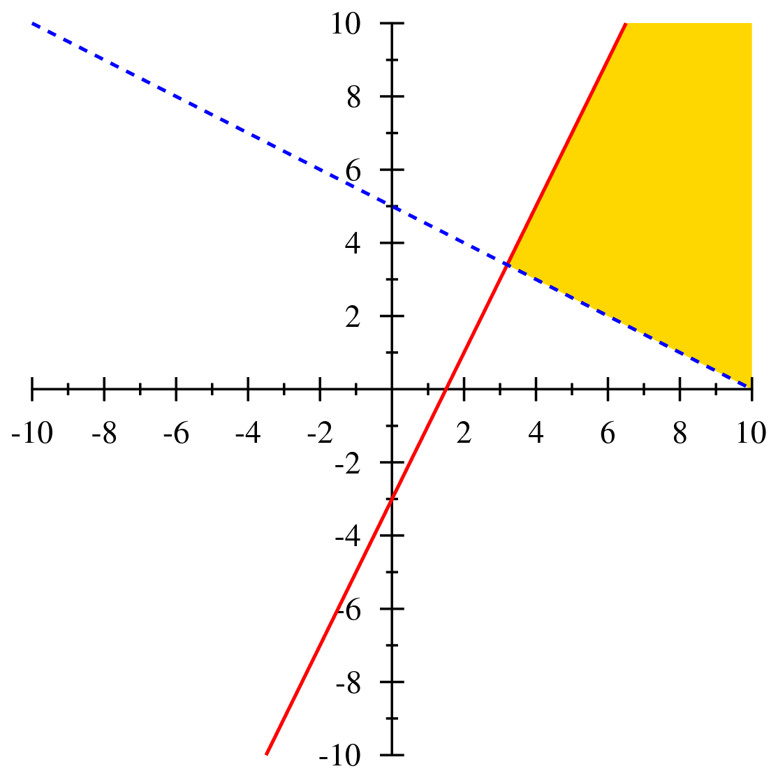

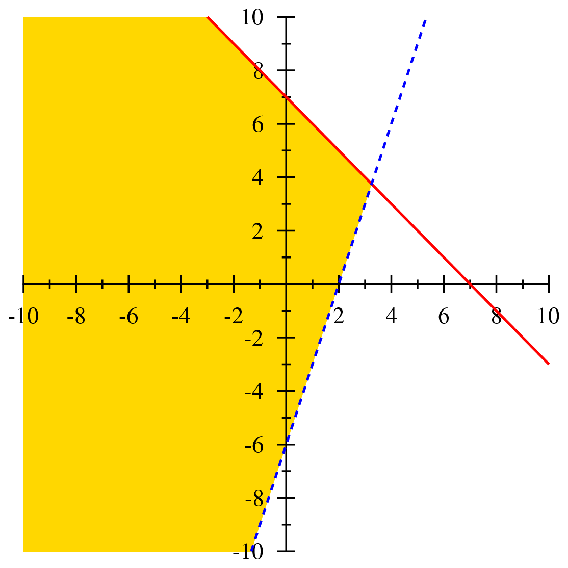
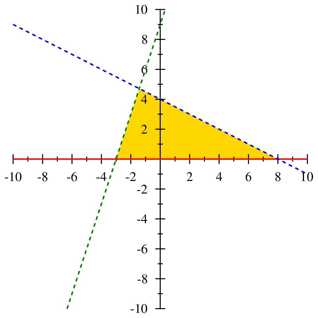
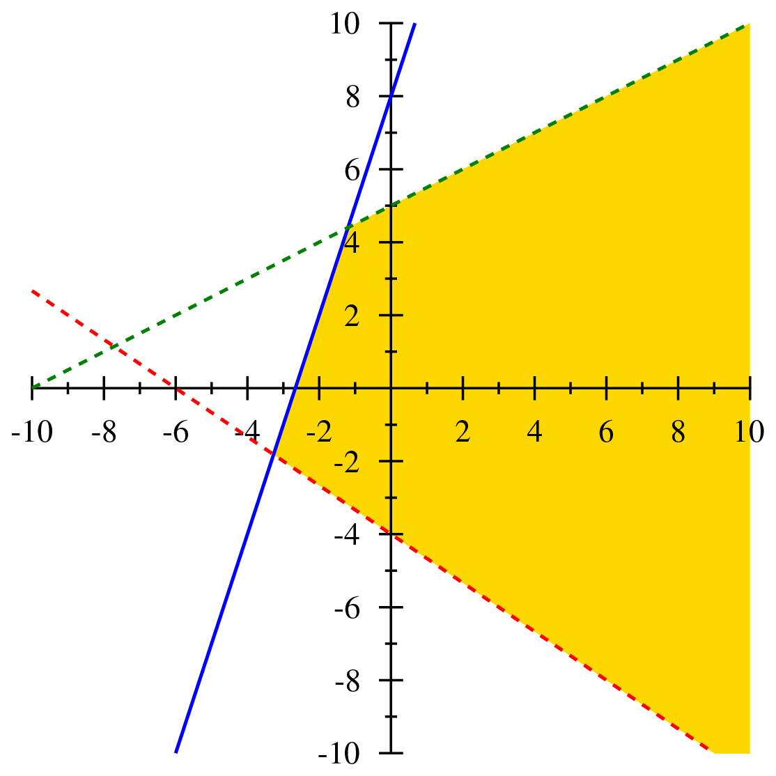
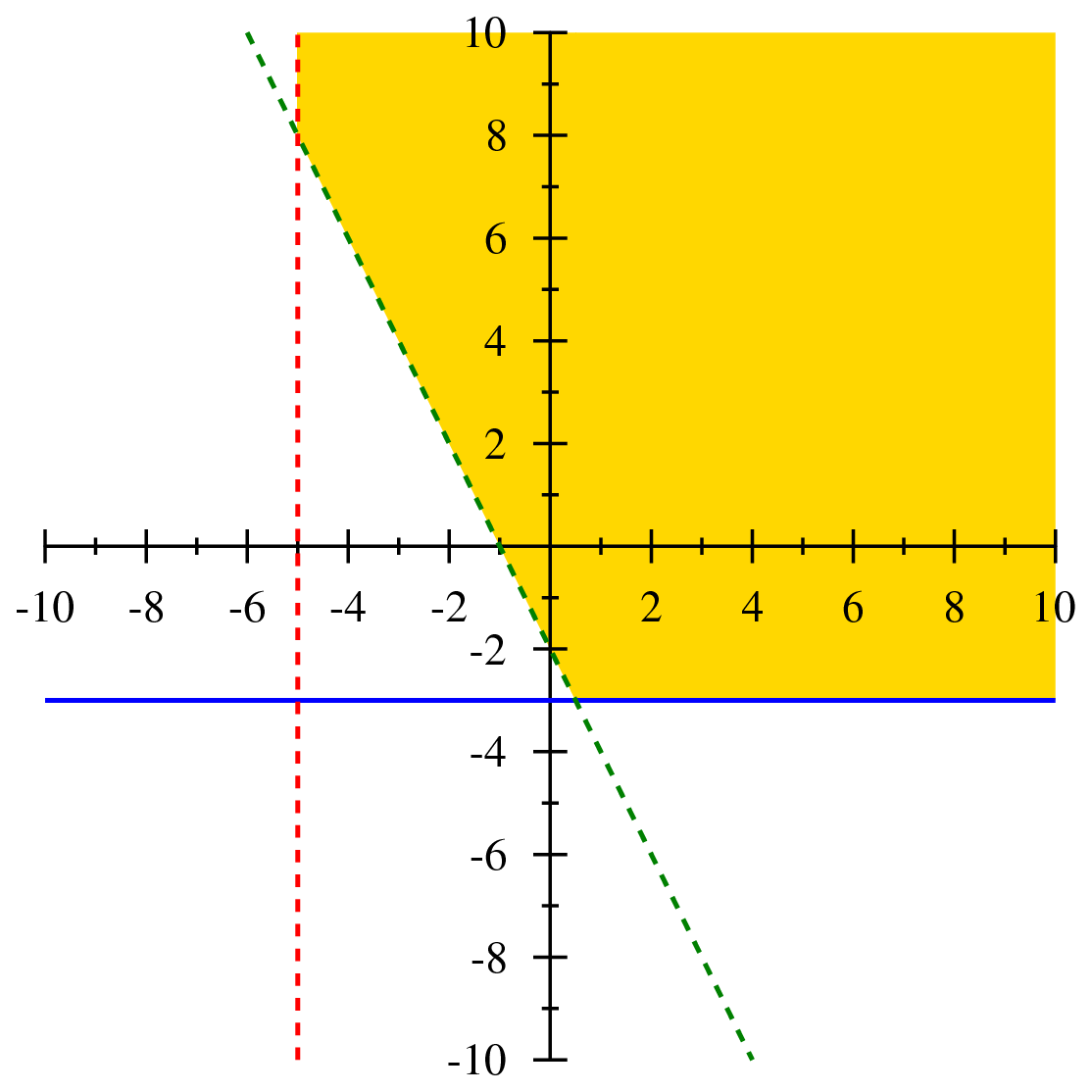
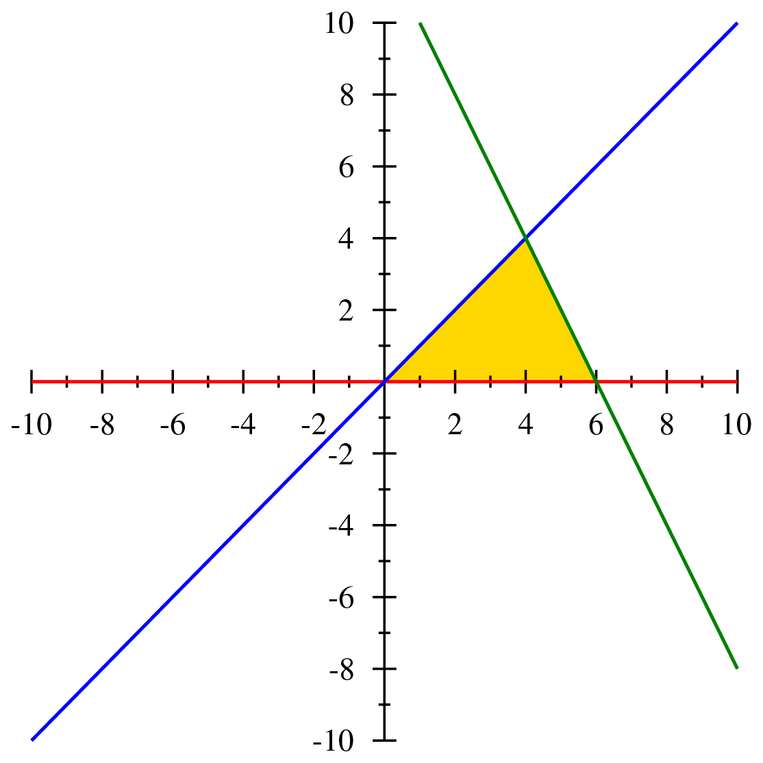
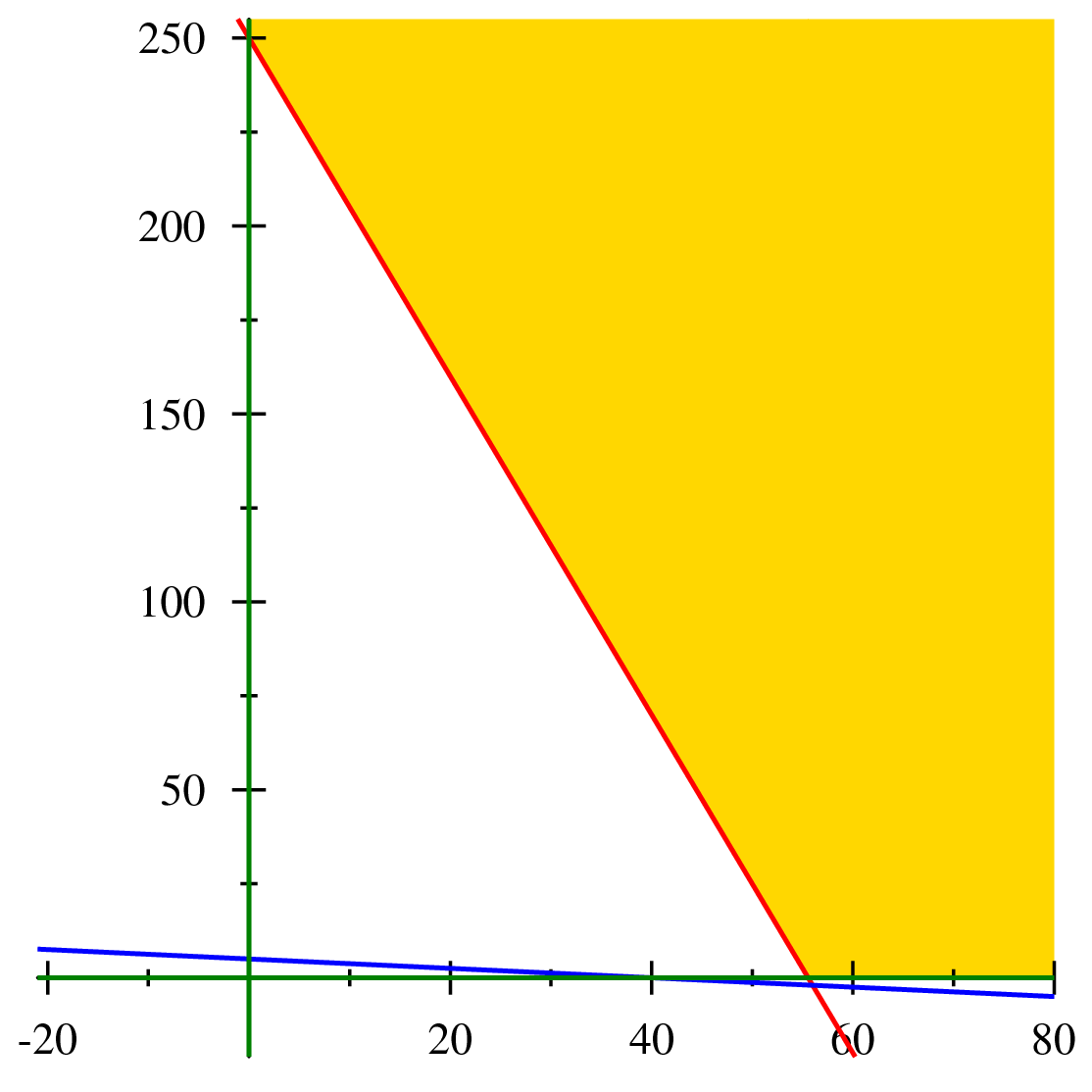
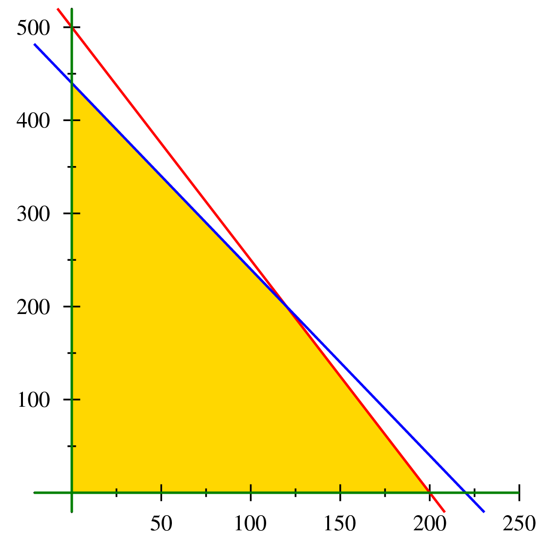


3 answers
Sun Jul 24, 2016 1:59 PM
Post by Joshua Jacob on July 23, 2014
Professor Vincent,
Could you explain the second equation in blue for example 2?
I graphed it out and even graphed it in my calculator and the shaded area is under the line, not above it.
Thanks for the amazing lectures!
Josh