


 Carleen Eaton
 Grant Fraser

Dr. Carleen Eaton
Solving Systems of Equations by Graphing
Slide Duration:Table of Contents
Section 1: Equations and Inequalities
Expressions and Formulas
22m 23s
- Intro0:00
- Order of Operations0:19
- Variable0:27
- Algebraic Expression0:46
- Term0:57
- Example: Algebraic Expression1:25
- Evaluate Inside Grouping Symbols1:55
- Evaluate Powers2:30
- Multiply/Divide Left to Right2:55
- Add/Subtract Left to Right3:35
- Monomials4:40
- Examples of Monomials4:52
- Constant5:27
- Coefficient5:46
- Degree6:25
- Power7:15
- Polynomials8:02
- Examples of Polynomials8:24
- Binomials, Trinomials, Monomials8:53
- Term9:21
- Like Terms10:02
- Formulas11:00
- Example: Pythagorean Theorem11:15
- Example 1: Evaluate the Algebraic Expression11:50
- Example 2: Evaluate the Algebraic Expression14:38
- Example 3: Area of a Triangle19:11
- Example 4: Fahrenheit to Celsius20:41
Properties of Real Numbers
20m 15s
- Intro0:00
- Real Numbers0:07
- Number Line0:15
- Rational Numbers0:46
- Irrational Numbers2:24
- Venn Diagram of Real Numbers4:03
- Irrational Numbers5:00
- Rational Numbers5:19
- Real Number System5:27
- Natural Numbers5:32
- Whole Numbers5:53
- Integers6:19
- Fractions6:46
- Properties of Real Numbers7:15
- Commutative Property7:34
- Associative Property8:07
- Identity Property9:04
- Inverse Property9:53
- Distributive Property11:03
- Example 1: What Set of Numbers?12:21
- Example 2: What Properties Are Used?13:56
- Example 3: Multiplicative Inverse16:00
- Example 4: Simplify Using Properties17:18
Solving Equations
19m 10s
- Intro0:00
- Translations0:06
- Verbal Expressions and Algebraic Expressions0:13
- Example: Sum of Two Numbers0:19
- Example: Square of a Number1:33
- Properties of Equality3:20
- Reflexive Property3:30
- Symmetric Property3:42
- Transitive Property4:01
- Addition Property5:01
- Subtraction Property5:37
- Multiplication Property6:02
- Division Property6:30
- Solving Equations6:58
- Example: Using Properties7:18
- Solving for a Variable8:25
- Example: Solve for Z8:34
- Example 1: Write Algebraic Expression10:15
- Example 2: Write Verbal Expression11:31
- Example 3: Solve the Equation14:05
- Example 4: Simplify Using Properties17:26
Solving Absolute Value Equations
17m 31s
- Intro0:00
- Absolute Value Expressions0:09
- Distance from Zero0:18
- Example: Absolute Value Expression0:24
- Absolute Value Equations1:50
- Example: Absolute Value Equation2:00
- Example: Isolate Expression3:13
- No Solution3:46
- Empty Set3:58
- Example: No Solution4:12
- Number of Solutions4:46
- Check Each Solution4:57
- Example: Two Solutions5:05
- Example: No Solution6:18
- Example: One Solution6:28
- Example 1: Evaluate for X7:16
- Example 2: Write Verbal Expression9:08
- Example 3: Solve the Equation12:18
- Example 4: Simplify Using Properties13:36
Solving Inequalities
17m 14s
- Intro0:00
- Properties of Inequalities0:08
- Addition Property0:17
- Example: Using Numbers0:30
- Subtraction Property1:03
- Example: Using Numbers1:19
- Multiplication Properties1:44
- C>0 (Positive Number)1:50
- Example: Using Numbers2:05
- C<0 (Negative Number)2:40
- Example: Using Numbers3:10
- Division Properties4:11
- C>0 (Positive Number)4:15
- Example: Using Numbers4:27
- C<0 (Negative Number)5:21
- Example: Using Numbers5:32
- Describing the Solution Set6:10
- Example: Set Builder Notation6:26
- Example: Graph (Closed Circle)7:08
- Example: Graph (Open Circle)7:30
- Example 1: Solve the Inequality7:58
- Example 2: Solve the Inequality9:06
- Example 3: Solve the Inequality10:10
- Example 4: Solve the Inequality13:12
Solving Compound and Absolute Value Inequalities
25m
- Intro0:00
- Compound Inequalities0:08
- And and Or0:13
- Example: And0:22
- Example: Or1:12
- And Inequality1:41
- Intersection1:49
- Example: Numbers2:08
- Example: Inequality2:43
- Or Inequality4:35
- Example: Union4:45
- Example: Inequality5:53
- Absolute Value Inequalities7:19
- Definition of Absolute Value7:33
- Examples: Compound Inequalities8:30
- Example: Complex Inequality12:21
- Example 1: Solve the Inequality12:54
- Example 2: Solve the Inequality17:21
- Example 3: Solve the Inequality18:54
- Example 4: Solve the Inequality22:15
Section 2: Linear Relations and Functions
Relations and Functions
32m 5s
- Intro0:00
- Coordinate Plane0:20
- X-Coordinate and Y-Coordinate0:30
- Example: Coordinate Pairs0:37
- Quadrants1:20
- Relations2:14
- Domain and Range2:19
- Set of Ordered Pairs2:29
- As a Table2:51
- Functions4:21
- One Element in Range4:32
- Example: Mapping4:43
- Example: Table and Map6:26
- One-to-One Functions8:01
- Example: One-to-One8:22
- Example: Not One-to-One9:18
- Graphs of Relations11:01
- Discrete and Continuous11:12
- Example: Discrete11:22
- Example: Continous12:30
- Vertical Line Test14:09
- Example: S Curve14:29
- Example: Function16:15
- Equations, Relations, and Functions17:03
- Independent Variable and Dependent Variable17:16
- Function Notation19:11
- Example: Function Notation19:23
- Example 1: Domain and Range20:51
- Example 2: Discrete or Continous23:03
- Example 3: Discrete or Continous25:53
- Example 4: Function Notation30:05
Linear Equations
14m 46s
- Intro0:00
- Linear Equations and Functions0:07
- Linear Equation0:19
- Example: Linear Equation0:29
- Example: Linear Function1:07
- Standard Form2:02
- Integer Constants with No Common Factor2:08
- Example: Standard Form2:27
- Graphing with Intercepts4:05
- X-Intercept and Y-Intercept4:12
- Example: Intercepts4:26
- Example: Graphing5:14
- Example 1: Linear Function7:53
- Example 2: Linear Function9:10
- Example 3: Standard Form10:04
- Example 4: Graph with Intercepts12:25
Slope
23m 7s
- Intro0:00
- Definition of Slope0:07
- Change in Y / Change in X0:26
- Example: Slope of Graph0:37
- Interpretation of Slope3:07
- Horizontal Line (0 Slope)3:13
- Vertical Line (Undefined Slope)4:52
- Rises to Right (Positive Slope)6:36
- Falls to Right (Negative Slope)6:53
- Parallel Lines7:18
- Example: Not Vertical7:30
- Example: Vertical7:58
- Perpendicular Lines8:31
- Example: Perpendicular8:42
- Example 1: Slope of Line10:32
- Example 2: Graph Line11:45
- Example 3: Parallel to Graph13:37
- Example 4: Perpendicular to Graph17:57
Writing Linear Functions
23m 5s
- Intro0:00
- Slope Intercept Form0:11
- m and b0:28
- Example: Graph Using Slope Intercept0:43
- Point Slope Form2:41
- Relation to Slope Formula3:03
- Example: Point Slope Form4:36
- Parallel and Perpendicular Lines6:28
- Review of Parallel and Perpendicular Lines6:31
- Example: Parallel7:50
- Example: Perpendicular9:58
- Example 1: Slope Intercept Form11:07
- Example 2: Slope Intercept Form13:07
- Example 3: Parallel15:49
- Example 4: Perpendicular18:42
Special Functions
31m 5s
- Intro0:00
- Step Functions0:07
- Example: Apple Prices0:30
- Absolute Value Function4:55
- Example: Absolute Value5:05
- Piecewise Functions9:08
- Example: Piecewise9:27
- Example 1: Absolute Value Function14:00
- Example 2: Absolute Value Function20:39
- Example 3: Piecewise Function22:26
- Example 4: Step Function25:25
Graphing Inequalities
21m 42s
- Intro0:00
- Graphing Linear Inequalities0:07
- Shaded Region0:19
- Using Test Points0:32
- Graph Corresponding Linear Function0:46
- Dashed or Solid Lines0:59
- Use Test Point1:21
- Example: Linear Inequality1:58
- Graphing Absolute Value Inequalities4:50
- Graph Corresponding Equations4:59
- Use Test Point5:20
- Example: Absolute Value Inequality5:38
- Example 1: Linear Inequality9:17
- Example 2: Linear Inequality11:56
- Example 3: Linear Inequality14:29
- Example 4: Absolute Value Inequality17:06
Section 3: Systems of Equations and Inequalities
Solving Systems of Equations by Graphing
17m 13s
- Intro0:00
- Systems of Equations0:09
- Example: Two Equations0:24
- Solving by Graphing0:53
- Point of Intersection1:09
- Types of Systems2:29
- Independent (Single Solution)2:34
- Dependent (Infinite Solutions)3:05
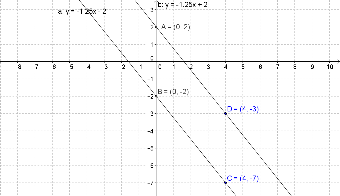
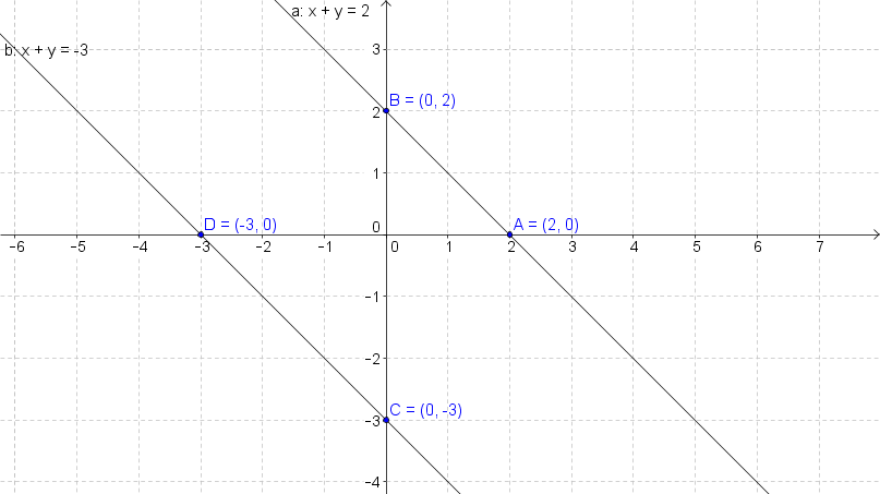
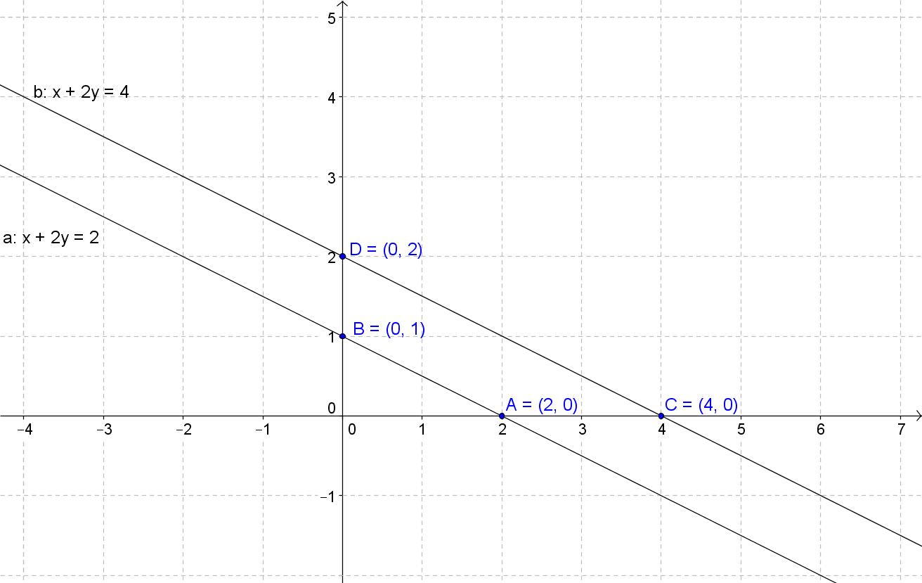
- Inconsistent (No Solution)4:23
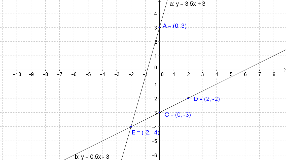
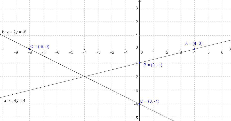
- Example 1: Solve by Graphing5:20
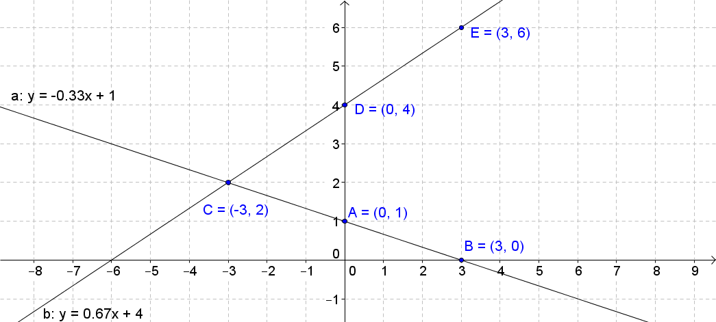
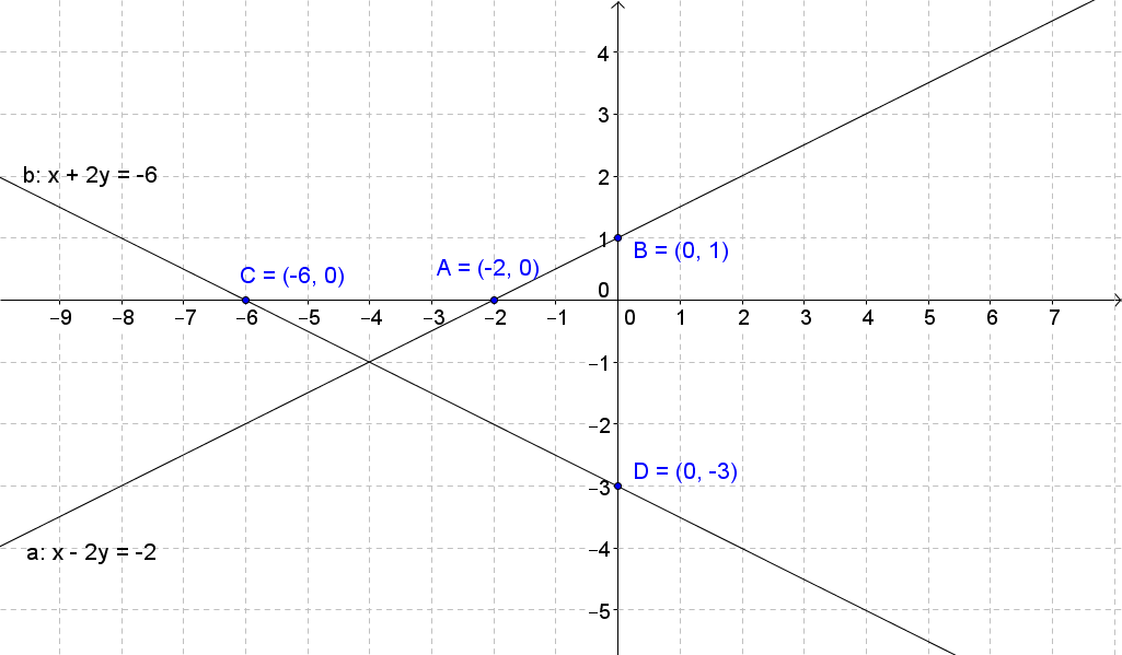
- Example 2: Solve by Graphing9:10
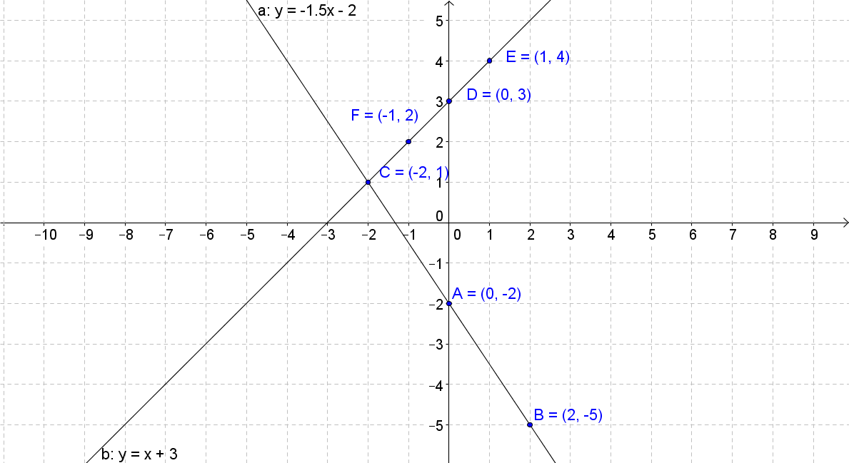
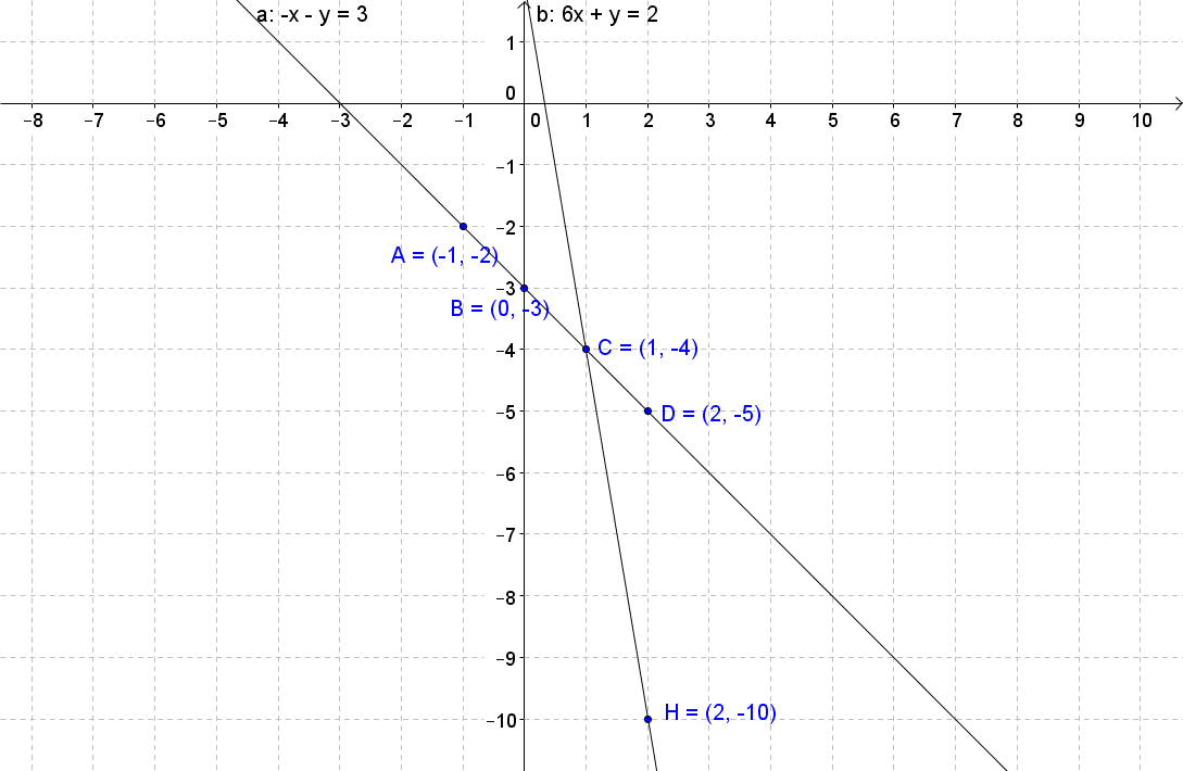
- Example 3: Solve by Graphing12:27
- Example 4: Solve by Graphing14:54
Solving Systems of Equations Algebraically
23m 53s
- Intro0:00
- Solving by Substitution0:08
- Example: System of Equations0:36
- Solving by Multiplication7:22
- Extra Step of Multiplying7:38
- Example: System of Equations8:00
- Inconsistent and Dependent Systems11:14
- Variables Drop Out11:48
- Inconsistent System (Never True)12:01
- Constant Equals Constant12:53
- Dependent System (Always True)13:11
- Example 1: Solve Algebraically13:58
- Example 2: Solve Algebraically15:52
- Example 3: Solve Algebraically17:54
- Example 4: Solve Algebraically21:40
Solving Systems of Inequalities By Graphing
27m 12s
- Intro0:00
- Solving by Graphing0:08
- Graph Each Inequality0:25
- Overlap0:35
- Corresponding Linear Equations1:03
- Test Point1:23
- Example: System of Inequalities1:51
- No Solution7:06
- Empty Set7:26
- Example: No Solution7:34
- Example 1: Solve by Graphing10:27
- Example 2: Solve by Graphing13:30
- Example 3: Solve by Graphing17:19
- Example 4: Solve by Graphing23:23
Solving Systems of Equations in Three Variables
28m 53s
- Intro0:00
- Solving Systems in Three Variables0:17
- Triple of Values0:31
- Example: Three Variables0:56
- Number of Solutions5:55
- One Solution6:08
- No Solution6:24
- Infinite Solutions7:06
- Example 1: Solve 3 Variables7:59
- Example 2: Solve 3 Variables13:50
- Example 3: Solve 3 Variables19:54
- Example 4: Solve 3 Variables25:50
Section 4: Matrices
Basic Matrix Concepts
11m 34s
- Intro0:00
- What is a Matrix0:26
- Brackets0:46
- Designation1:21
- Element1:47
- Matrix Equations1:59
- Dimensions2:27
- Rows (m) and Columns (n)2:37
- Examples: Dimensions2:43
- Special Matrices4:22
- Row Matrix4:32
- Column Matrix5:00
- Zero Matrix6:00
- Equal Matrices6:30
- Example: Corresponding Elements6:36
- Example 1: Matrix Dimension8:12
- Example 2: Matrix Dimension9:03
- Example 3: Zero Matrix9:38
- Example 4: Row and Column Matrix10:26
Matrix Operations
21m 36s
- Intro0:00
- Matrix Addition0:18
- Same Dimensions0:25
- Example: Adding Matrices1:04
- Matrix Subtraction3:42
- Same Dimensions3:48
- Example: Subtracting Matrices4:04
- Scalar Multiplication6:08
- Scalar Constant6:24
- Example: Multiplying Matrices6:32
- Properties of Matrix Operations8:23
- Commutative Property8:41
- Associative Property9:08
- Distributive Property9:44
- Example 1: Matrix Addition10:24
- Example 2: Matrix Subtraction11:58
- Example 3: Scalar Multiplication14:23
- Example 4: Matrix Properties16:09
Matrix Multiplication
29m 36s
- Intro0:00
- Dimension Requirement0:17
- n = p0:24
- Resulting Product Matrix (m x q)1:21
- Example: Multiplication1:54
- Matrix Multiplication3:38
- Example: Matrix Multiplication4:07
- Properties of Matrix Multiplication10:46
- Associative Property11:00
- Associative Property (Scalar)11:28
- Distributive Property12:06
- Distributive Property (Scalar)12:30
- Example 1: Possible Matrices13:31
- Example 2: Multiplying Matrices17:08
- Example 3: Multiplying Matrices20:41
- Example 4: Matrix Properties24:41
Determinants
33m 13s
- Intro0:00
- What is a Determinant0:13
- Square Matrices0:23
- Vertical Bars0:41
- Determinant of a 2x2 Matrix1:21
- Second Order Determinant1:37
- Formula1:45
- Example: 2x2 Determinant1:58
- Determinant of a 3x3 Matrix2:50
- Expansion by Minors3:08
- Third Order Determinant3:19
- Expanding Row One4:06
- Example: 3x3 Determinant6:40
- Diagonal Method for 3x3 Matrices13:24
- Example: Diagonal Method13:36
- Example 1: Determinant of 2x218:59
- Example 2: Determinant of 3x320:03
- Example 3: Determinant of 3x325:35
- Example 4: Determinant of 3x329:22
Cramer's Rule
28m 25s
- Intro0:00
- System of Two Equations in Two Variables0:16
- One Variable0:50
- Determinant of Denominator1:14
- Determinants of Numerators2:23
- Example: System of Equations3:34
- System of Three Equations in Three Variables7:06
- Determinant of Denominator7:17
- Determinants of Numerators7:52
- Example 1: Two Equations8:57
- Example 2: Two Equations13:21
- Example 3: Three Equations17:11
- Example 4: Three Equations23:43
Identity and Inverse Matrices
22m 25s
- Intro0:00
- Identity Matrix0:13
- Example: 2x2 Identity Matrix0:30
- Example: 4x4 Identity Matrix0:50
- Properties of Identity Matrices1:24
- Example: Multiplying Identity Matrix2:52
- Matrix Inverses5:30
- Writing Matrix Inverse6:07
- Inverse of a 2x2 Matrix6:39
- Example: 2x2 Matrix7:31
- Example 1: Inverse Matrix10:18
- Example 2: Find the Inverse Matrix13:04
- Example 3: Find the Inverse Matrix17:53
- Example 4: Find the Inverse Matrix20:44
Solving Systems of Equations Using Matrices
22m 32s
- Intro0:00
- Matrix Equations0:11
- Example: System of Equations0:21
- Solving Systems of Equations4:01
- Isolate x4:16
- Example: Using Numbers5:10
- Multiplicative Inverse5:54
- Example 1: Write as Matrix Equation7:18
- Example 2: Use Matrix Equations9:12
- Example 3: Use Matrix Equations15:06
- Example 4: Use Matrix Equations19:35
Section 5: Quadratic Functions and Inequalities
Graphing Quadratic Functions
31m 48s
- Intro0:00
- Quadratic Functions0:12
- A is Zero0:27
- Example: Parabola0:45
- Properties of Parabolas2:08
- Axis of Symmetry2:11
- Vertex2:32
- Example: Parabola2:48
- Minimum and Maximum Values9:02
- Positive or Negative9:28
- Upward or Downward9:58
- Example: Minimum10:31
- Example: Maximum11:16
- Example 1: Axis of Symmetry, Vertex, Graph12:41
- Example 2: Axis of Symmetry, Vertex, Graph17:25
- Example 3: Minimum or Maximum21:47
- Example 4: Minimum or Maximum27:09
Solving Quadratic Equations by Graphing
27m 3s
- Intro0:00
- Quadratic Equations0:16
- Standard Form0:18
- Example: Quadratic Equation0:47
- Solving by Graphing1:41
- Roots (x-Intercepts)1:48
- Example: Number of Solutions2:12
- Estimating Solutions9:23
- Example: Integer Solutions9:30
- Example: Estimating9:53
- Example 1: Solve by Graphing10:52
- Example 2: Solve by Graphing15:10
- Example 1: Solve by Graphing17:50
- Example 1: Solve by Graphing20:54
Solving Quadratic Equations by Factoring
19m 53s
- Intro0:00
- Factoring Techniques0:15
- Greatest Common Factor (GCF)0:37
- Difference of Two Squares1:48
- Perfect Square Trinomials2:30
- General Trinomials3:09
- Zero Product Rule5:22
- Example: Zero Product5:53
- Example 1: Solve by Factoring7:46
- Example 1: Solve by Factoring9:48
- Example 1: Solve by Factoring12:34
- Example 1: Solve by Factoring15:28
Imaginary and Complex Numbers
35m 45s
- Intro0:00
- Properties of Square Roots0:10
- Product Property0:26
- Example: Product Property0:56
- Quotient Property2:17
- Example: Quotient Property2:35
- Imaginary Numbers3:12
- Imaginary i3:51
- Examples: Imaginary Number4:22
- Complex Numbers7:23
- Real Part and Imaginary Part7:33
- Examples: Complex Numbers7:57
- Equality9:37
- Example: Equal Complex Numbers9:52
- Addition and Subtraction10:12
- Examples: Adding Complex Numbers10:25
- Complex Plane13:32
- Horizontal Axis (Real)13:49
- Vertical Axis (Imaginary)13:59
- Example: Labeling14:11
- Multiplication15:57
- Example: FOIL Method16:03
- Division18:37
- Complex Conjugates18:45
- Conjugate Pairs19:10
- Example: Dividing Complex Numbers20:00
- Example 1: Simplify Complex Number24:50
- Example 2: Simplify Complex Number27:56
- Example 3: Multiply Complex Numbers29:27
- Example 3: Dividing Complex Numbers31:48
Completing the Square
27m 11s
- Intro0:00
- Square Root Property0:12
- Example: Perfect Square0:38
- Example: Perfect Square Trinomial3:00
- Completing the Square4:39
- Constant Term4:50
- Example: Complete the Square5:04
- Solve Equations6:42
- Add to Both Sides6:59
- Example: Complete the Square7:07
- Equations Where a Not Equal to 110:58
- Divide by Coefficient11:08
- Example: Complete the Square11:24
- Complex Solutions14:05
- Real and Imaginary14:14
- Example: Complex Solution14:35
- Example 1: Square Root Property18:31
- Example 2: Complete the Square19:15
- Example 3: Complete the Square20:40
- Example 4: Complete the Square23:56
Quadratic Formula and the Discriminant
22m 48s
- Intro0:00
- Quadratic Formula0:21
- Standard Form0:29
- Example: Quadratic Formula0:57
- One Rational Root3:00
- Example: One Root3:31
- Complex Solutions6:16
- Complex Conjugate6:28
- Example: Complex Solution7:15
- Discriminant9:42
- Positive Discriminant10:03
- Perfect Square (Rational)10:51
- Not Perfect Square (2 Irrational)11:27
- Negative Discriminant12:28
- Zero Discriminant12:57
- Example 1: Quadratic Formula13:50
- Example 2: Quadratic Formula16:03
- Example 3: Quadratic Formula19:00
- Example 4: Discriminant21:33
Analyzing the Graphs of Quadratic Functions
30m 7s
- Intro0:00
- Vertex Form0:12
- H and K0:32
- Axis of Symmetry0:36
- Vertex0:42
- Example: Origin1:00
- Example: k = 22:12
- Example: h = 14:27
- Significance of Coefficient a7:13
- Example: |a| > 17:25
- Example: |a| < 18:18
- Example: |a| > 08:51
- Example: |a| < 09:05
- Writing Quadratic Equations in Vertex Form10:22
- Standard Form to Vertex Form10:35
- Example: Standard Form11:02
- Example: a Term Not 114:42
- Example 1: Vertex Form19:47
- Example 2: Vertex Form22:09
- Example 3: Vertex Form24:32
- Example 4: Vertex Form28:23
Graphing and Solving Quadratic Inequalities
27m 5s
- Intro0:00
- Graphing Quadratic Inequalities0:11
- Test Point0:18
- Example: Quadratic Inequality0:29
- Solving Quadratic Inequalities3:57
- Example: Parameter4:24
- Example 1: Graph Inequality11:16
- Example 2: Solve Inequality14:27
- Example 3: Graph Inequality19:14
- Example 4: Solve Inequality23:48
Section 6: Polynomial Functions
Properties of Exponents
19m 29s
- Intro0:00
- Simplifying Exponential Expressions0:09
- Monomial Simplest Form0:19
- Negative Exponents1:07
- Examples: Simple1:34
- Properties of Exponents3:06
- Negative Exponents3:13
- Mutliplying Same Base3:24
- Dividing Same Base3:45
- Raising Power to a Power4:33
- Parentheses (Multiplying)5:11
- Parentheses (Dividing)5:47
- Raising to 0th Power6:15
- Example 1: Simplify Exponents7:59
- Example 2: Simplify Exponents10:41
- Example 3: Simplify Exponents14:11
- Example 4: Simplify Exponents18:04
Operations on Polynomials
13m 27s
- Intro0:00
- Adding and Subtracting Polynomials0:13
- Like Terms and Like Monomials0:23
- Examples: Adding Monomials1:14
- Multiplying Polynomials3:40
- Distributive Property3:44
- Example: Monomial by Polynomial4:06
- Example 1: Simplify Polynomials5:47
- Example 2: Simplify Polynomials6:28
- Example 3: Simplify Polynomials8:38
- Example 4: Simplify Polynomials10:47
Dividing Polynomials
31m 11s
- Intro0:00
- Dividing by a Monomial0:13
- Example: Numbers0:26
- Example: Polynomial by a Monomial1:18
- Long Division2:28
- Remainder Term2:41
- Example: Dividing with Numbers3:04
- Example: With Polynomials5:01
- Example: Missing Terms7:58
- Synthetic Division11:44
- Restriction12:04
- Example: Divisor in Form12:20
- Divisor in Synthetic Division15:54
- Example: Coefficient to 116:07
- Example 1: Divide Polynomials17:10
- Example 2: Divide Polynomials19:08
- Example 3: Synthetic Division21:42
- Example 4: Synthetic Division25:09
Polynomial Functions
22m 30s
- Intro0:00
- Polynomial in One Variable0:13
- Leading Coefficient0:27
- Example: Polynomial1:18
- Degree1:31
- Polynomial Functions2:57
- Example: Function3:13
- Function Values3:33
- Example: Numerical Values3:53
- Example: Algebraic Expressions5:11
- Zeros of Polynomial Functions5:50
- Odd Degree6:04
- Even Degree7:29
- End Behavior8:28
- Even Degrees9:09
- Example: Leading Coefficient +/-9:23
- Odd Degrees12:51
- Example: Leading Coefficient +/-13:00
- Example 1: Degree and Leading Coefficient15:03
- Example 2: Polynomial Function15:56
- Example 3: Polynomial Function17:34
- Example 4: End Behavior19:53
Analyzing Graphs of Polynomial Functions
33m 29s
- Intro0:00
- Graphing Polynomial Functions0:11
- Example: Table and End Behavior0:39
- Location Principle4:43
- Zero Between Two Points5:03
- Example: Location Principle5:21
- Maximum and Minimum Points8:40
- Relative Maximum and Relative Minimum9:16
- Example: Number of Relative Max/Min11:11
- Example 1: Graph Polynomial Function11:57
- Example 2: Graph Polynomial Function16:19
- Example 3: Graph Polynomial Function23:27
- Example 4: Graph Polynomial Function28:35
Solving Polynomial Functions
21m 10s
- Intro0:00
- Factoring Polynomials0:06
- Greatest Common Factor (GCF)0:25
- Difference of Two Squares1:14
- Perfect Square Trinomials2:07
- General Trinomials2:57
- Grouping4:32
- Sum and Difference of Two Cubes6:03
- Examples: Two Cubes6:14
- Quadratic Form8:22
- Example: Quadratic Form8:44
- Example 1: Factor Polynomial12:03
- Example 2: Factor Polynomial13:54
- Example 3: Quadratic Form15:33
- Example 4: Solve Polynomial Function17:24
Remainder and Factor Theorems
31m 21s
- Intro0:00
- Remainder Theorem0:07
- Checking Work0:22
- Dividend and Divisor in Theorem1:12
- Example: f(a)2:05
- Synthetic Substitution5:43
- Example: Polynomial Function6:15
- Factor Theorem9:54
- Example: Numbers10:16
- Example: Confirm Factor11:27
- Factoring Polynomials14:48
- Example: 3rd Degree Polynomial15:07
- Example 1: Remainder Theorem19:17
- Example 2: Other Factors21:57
- Example 3: Remainder Theorem25:52
- Example 4: Other Factors28:21
Roots and Zeros
31m 27s
- Intro0:00
- Number of Roots0:08
- Not Nature of Roots0:18
- Example: Real and Complex Roots0:25
- Descartes' Rule of Signs2:05
- Positive Real Roots2:21
- Example: Positve2:39
- Negative Real Roots5:44
- Example: Negative6:06
- Finding the Roots9:59
- Example: Combination of Real and Complex10:07
- Conjugate Roots13:18
- Example: Conjugate Roots13:50
- Example 1: Solve Polynomial16:03
- Example 2: Solve Polynomial18:36
- Example 3: Possible Combinations23:13
- Example 4: Possible Combinations27:11
Rational Zero Theorem
31m 16s
- Intro0:00
- Equation0:08
- List of Possibilities0:16
- Equation with Constant and Leading Coefficient1:04
- Example: Rational Zero2:46
- Leading Coefficient Equal to One7:19
- Equation with Leading Coefficient of One7:34
- Example: Coefficient Equal to 18:45
- Finding Rational Zeros12:58
- Division with Remainder Zero13:32
- Example 1: Possible Rational Zeros14:20
- Example 2: Possible Rational Zeros16:02
- Example 3: Possible Rational Zeros19:58
- Example 4: Find All Zeros22:06
Section 7: Radical Expressions and Inequalities
Operations on Functions
34m 30s
- Intro0:00
- Arithmetic Operations0:07
- Domain0:16
- Intersection0:24
- Denominator is Zero0:49
- Example: Operations1:02
- Composition of Functions7:18
- Notation7:48
- Right to Left8:18
- Example: Composition8:48
- Composition is Not Commutative17:23
- Example: Not Commutative17:51
- Example 1: Function Operations20:55
- Example 2: Function Operations24:34
- Example 3: Compositions27:51
- Example 4: Function Operations31:09
Inverse Functions and Relations
22m 42s
- Intro0:00
- Inverse of a Relation0:14
- Example: Ordered Pairs0:56
- Inverse of a Function3:24
- Domain and Range Switched3:52
- Example: Inverse4:28
- Procedure to Construct an Inverse Function6:42
- f(x) to y6:42
- Interchange x and y6:59
- Solve for y7:06
- Write Inverse f(x) for y7:14
- Example: Inverse Function7:25
- Example: Inverse Function 28:48
- Inverses and Compositions10:44
- Example: Inverse Composition11:46
- Example 1: Inverse Relation14:49
- Example 2: Inverse of Function15:40
- Example 3: Inverse of Function17:06
- Example 4: Inverse Functions18:55
Square Root Functions and Inequalities
30m 4s
- Intro0:00
- Square Root Functions0:07
- Examples: Square Root Function0:16
- Example: Not Square Root Function0:46
- Radicand1:12
- Example: Restriction1:31
- Graphing Square Root Functions3:42
- Example: Graphing3:49
- Square Root Inequalities8:47
- Same Technique9:00
- Example: Square Root Inequality9:20
- Example 1: Graph Square Root Function15:19
- Example 2: Graph Square Root Function18:03
- Example 3: Graph Square Root Function22:41
- Example 4: Square Root Inequalities25:37
nth Roots
20m 46s
- Intro0:00
- Definition of the nth Root0:07
- Example: 5th Root0:20
- Example: 6th Root0:51
- Principal nth Root1:39
- Example: Principal Roots2:06
- Using Absolute Values5:58
- Example: Square Root6:18
- Example: 6th Root8:40
- Example: Negative10:15
- Example 1: Simplify Radicals12:23
- Example 2: Simplify Radicals13:29
- Example 3: Simplify Radicals16:07
- Example 4: Simplify Radicals18:18
Operations with Radical Expressions
41m 11s
- Intro0:00
- Properties of Radicals0:16
- Quotient Property0:29
- Example: Quotient1:00
- Example: Product Property1:47
- Simplifying Radical Expressions3:24
- Radicand No nth Powers3:47
- Radicand No Fractions6:33
- No Radicals in Denominator7:16
- Rationalizing Denominators8:27
- Example: Radicand nth Power9:05
- Conjugate Radical Expressions11:47
- Conjugates12:07
- Example: Conjugate Radical Expression13:11
- Adding and Subtracting Radicals16:12
- Same Index, Same Radicand16:20
- Example: Like Radicals16:28
- Multiplying Radicals19:04
- Distributive Property19:10
- Example: Multiplying Radicals19:20
- Example 1: Simplify Radical24:11
- Example 2: Simplify Radicals28:43
- Example 3: Simplify Radicals32:00
- Example 4: Simplify Radical36:34
Rational Exponents
30m 45s
- Intro0:00
- Definition 10:20
- Example: Using Numbers0:39
- Example: Non-Negative2:46
- Example: Odd3:34
- Definition 24:32
- Restriction4:52
- Example: Relate to Definition 15:04
- Example: m Not 15:31
- Simplifying Expressions7:53
- Multiplication8:31
- Division9:29
- Multiply Exponents10:08
- Raised Power11:05
- Zero Power11:29
- Negative Power11:49
- Simplified Form13:52
- Complex Fraction14:16
- Negative Exponents14:40
- Example: More Complicated15:14
- Example 1: Write as Radical19:03
- Example 2: Write with Rational Exponents20:40
- Example 3: Complex Fraction22:09
- Example 4: Complex Fraction26:22
Solving Radical Equations and Inequalities
31m 27s
- Intro0:00
- Radical Equations0:11
- Variables in Radicands0:22
- Example: Radical Equation1:06
- Example: Complex Equation2:42
- Extraneous Roots7:21
- Squaring Technique7:35
- Double Check7:44
- Example: Extraneous8:21
- Eliminating nth Roots10:04
- Isolate and Raise Power10:14
- Example: nth Root10:27
- Radical Inequalities11:27
- Restriction: Index is Even11:53
- Example: Radical Inequality12:29
- Example 1: Solve Radical Equation15:41
- Example 2: Solve Radical Equation17:44
- Example 3: Solve Radical Inequality20:24
- Example 4: Solve Radical Equation24:34
Section 8: Rational Equations and Inequalities
Multiplying and Dividing Rational Expressions
40m 54s
- Intro0:00
- Simplifying Rational Expressions0:22
- Algebraic Fraction0:29
- Examples: Rational Expressions0:49
- Example: GCF1:33
- Example: Simplify Rational Expression2:26
- Factoring -14:04
- Example: Simplify with -14:19
- Multiplying and Dividing Rational Expressions6:59
- Multiplying and Dividing7:28
- Example: Multiplying Rational Expressions8:36
- Example: Dividing Rational Expressions11:20
- Factoring14:01
- Factoring Polynomials14:19
- Example: Factoring14:35
- Complex Fractions18:22
- Example: Numbers18:37
- Example: Algebraic Complex Fractions19:25
- Example 1: Simplify Rational Expression25:56
- Example 2: Simplify Rational Expression29:34
- Example 3: Simplify Rational Expression31:39
- Example 4: Simplify Rational Expression37:50
Adding and Subtracting Rational Expressions
55m 4s
- Intro0:00
- Least Common Multiple (LCM)0:27
- Examples: LCM of Numbers0:43
- Example: LCM of Polynomials4:02
- Adding and Subtracting7:55
- Least Common Denominator (LCD)8:07
- Example: Numbers8:17
- Example: Rational Expressions11:03
- Equivalent Fractions15:22
- Simplifying Complex Fractions21:19
- Example: Previous Lessons21:36
- Example: More Complex22:53
- Example 1: Find LCM28:30
- Example 2: Add Rational Expressions31:44
- Example 3: Subtract Rational Expressions39:18
- Example 4: Simplify Rational Expression38:26
Graphing Rational Functions
57m 13s
- Intro0:00
- Rational Functions0:18
- Restriction0:34
- Example: Rational Function0:51
- Breaks in Continuity2:52
- Example: Continuous Function3:10
- Discontinuities3:30
- Example: Excluded Values4:37
- Graphs and Discontinuities5:02
- Common Binomial Factor (Hole)5:08
- Example: Common Factor5:31
- Asymptote10:06
- Example: Vertical Asymptote11:08
- Horizontal Asymptotes20:00
- Example: Horizontal Asymptote20:25
- Example 1: Holes and Vertical Asymptotes26:12
- Example 2: Graph Rational Faction28:35
- Example 3: Graph Rational Faction39:23
- Example 4: Graph Rational Faction47:28
Direct, Joint, and Inverse Variation
20m 21s
- Intro0:00
- Direct Variation0:07
- Constant of Variation0:25
- Graph of Constant Variation1:26
- Slope is Constant k1:35
- Example: Straight Lines1:41
- Joint Variation2:48
- Three Variables2:52
- Inverse Variation3:38
- Rewritten Form3:52
- Examples in Biology4:22
- Graph of Inverse Variation4:51
- Asymptotes are Axes5:12
- Example: Inverse Variation5:40
- Proportions10:11
- Direct Variation10:25
- Inverse Variation11:32
- Example 1: Type of Variation12:42
- Example 2: Direct Variation14:13
- Example 3: Joint Variation16:24
- Example 4: Graph Rational Faction18:50
Solving Rational Equations and Inequalities
55m 14s
- Intro0:00
- Rational Equations0:15
- Example: Algebraic Fraction0:26
- Least Common Denominator0:49
- Example: Simple Rational Equation1:22
- Example: Solve Rational Equation5:40
- Extraneous Solutions9:31
- Doublecheck10:00
- No Solution10:38
- Example: Extraneous10:44
- Rational Inequalities14:01
- Excluded Values14:31
- Solve Related Equation14:49
- Find Intervals14:58
- Use Test Values15:25
- Example: Rational Inequality15:51
- Example: Rational Inequality 217:07
- Example 1: Rational Equation28:50
- Example 2: Rational Equation33:51
- Example 3: Rational Equation38:19
- Example 4: Rational Inequality46:49
Section 9: Exponential and Logarithmic Relations
Exponential Functions
35m 58s
- Intro0:00
- What is an Exponential Function?0:12
- Restriction on b0:31
- Base0:46
- Example: Exponents as Bases0:56
- Variables as Exponents1:12
- Example: Exponential Function1:50
- Graphing Exponential Functions2:33
- Example: Using Table2:49
- Properties11:52
- Continuous and One to One12:00
- Domain is All Real Numbers13:14
- X-Axis Asymptote13:55
- Y-Intercept14:02
- Reflection Across Y-Axis14:31
- Growth and Decay15:06
- Exponential Growth15:10
- Real Life Examples15:41
- Example: Growth15:52
- Example: Decay16:12
- Real Life Examples16:30
- Equations17:32
- Bases are Same18:05
- Examples: Variables as Exponents18:20
- Inequalities21:29
- Property21:51
- Example: Inequality22:37
- Example 1: Graph Exponential Function24:05
- Example 2: Growth or Decay27:50
- Example 3: Exponential Equation29:31
- Example 4: Exponential Inequality32:54
Logarithms and Logarithmic Functions
45m 54s
- Intro0:00
- What are Logarithms?0:08
- Restrictions0:15
- Written Form0:26
- Logarithms are Exponents0:52
- Example: Logarithms1:49
- Logarithmic Functions5:14
- Same Restrictions5:30
- Inverses5:53
- Example: Logarithmic Function6:24
- Graph of the Logarithmic Function9:20
- Example: Using Table9:35
- Properties15:09
- Continuous and One to One15:14
- Domain15:36
- Range15:56
- Y-Axis is Asymptote16:02
- X Intercept16:12
- Inverse Property16:57
- Compositions of Functions17:10
- Equations18:30
- Example: Logarithmic Equation19:13
- Inequalities20:36
- Properties20:47
- Example: Logarithmic Inequality21:40
- Equations with Logarithms on Both Sides24:43
- Property24:51
- Example: Both Sides25:23
- Inequalities with Logarithms on Both Sides26:52
- Property27:02
- Example: Both Sides28:05
- Example 1: Solve Log Equation31:52
- Example 2: Solve Log Equation33:53
- Example 3: Solve Log Equation36:15
- Example 4: Solve Log Inequality39:19
Properties of Logarithms
28m 43s
- Intro0:00
- Product Property0:08
- Example: Product0:46
- Quotient Property2:40
- Example: Quotient2:59
- Power Property3:51
- Moved Exponent4:07
- Example: Power4:37
- Equations5:15
- Example: Use Properties5:58
- Example 1: Simplify Log11:17
- Example 2: Single Log15:54
- Example 3: Solve Log Equation18:48
- Example 4: Solve Log Equation22:13
Common Logarithms
25m 23s
- Intro0:00
- What are Common Logarithms?0:10
- Real World Applications0:16
- Base Not Written0:27
- Example: Base 100:39
- Equations1:47
- Example: Same Base1:56
- Example: Different Base2:37
- Inequalities6:07
- Multiplying/Dividing Inequality6:21
- Example: Log Inequality6:54
- Change of Base12:45
- Base 1013:24
- Example: Change of Base14:05
- Example 1: Log Equation15:21
- Example 2: Common Logs17:13
- Example 3: Log Equation18:22
- Example 4: Log Inequality21:52
Base e and Natural Logarithms
21m 14s
- Intro0:00
- Number e0:09
- Natural Base0:21
- Growth/Decay0:33
- Example: Exponential Function0:53
- Natural Logarithms1:11
- ln x1:19
- Inverse and Identity Function1:39
- Example: Inverse Composition1:55
- Equations and Inequalities4:39
- Extraneous Solutions5:30
- Examples: Natural Log Equations5:48
- Example 1: Natural Log Equation9:08
- Example 2: Natural Log Equation10:37
- Example 3: Natural Log Inequality16:54
- Example 4: Natural Log Inequality18:16
Exponential Growth and Decay
24m 30s
- Intro0:00
- Decay0:17
- Decreases by Fixed Percentage0:23
- Rate of Decay0:56
- Example: Finance1:34
- Scientific Model of Decay3:37
- Exponential Decay3:45
- Radioactive Decay4:13
- Example: Half Life5:33
- Growth9:06
- Increases by Fixed Percentage9:18
- Example: Finance10:09
- Scientific Model of Growth11:35
- Population Growth12:04
- Example: Growth12:20
- Example 1: Computer Price14:00
- Example 2: Stock Price15:46
- Example 3: Medicine Disintegration19:10
- Example 4: Population Growth22:33
Section 10: Conic Sections
Midpoint and Distance Formulas
32m 42s
- Intro0:00
- Midpoint Formula0:15
- Example: Midpoint0:30
- Distance Formula2:30
- Example: Distance2:52
- Example 1: Midpoint and Distance4:58
- Example 2: Midpoint and Distance8:07
- Example 3: Median Length18:51
- Example 4: Perimeter and Area23:36
Parabolas
41m 27s
- Intro0:00
- What is a Parabola?0:20
- Definition of a Parabola0:29
- Focus0:59
- Directrix1:15
- Axis of Symmetry3:08
- Vertex3:33
- Minimum or Maximum3:44
- Standard Form4:59
- Horizontal Parabolas5:08
- Vertex Form5:19
- Upward or Downward5:41
- Example: Standard Form6:06
- Graphing Parabolas8:31
- Shifting8:51
- Example: Completing the Square9:22
- Symmetry and Translation12:18
- Example: Graph Parabola12:40
- Latus Rectum17:13
- Length18:15
- Example: Latus Rectum18:35
- Horizontal Parabolas18:57
- Not Functions20:08
- Example: Horizontal Parabola21:21
- Focus and Directrix24:11
- Horizontal24:48
- Example 1: Parabola Standard Form25:12
- Example 2: Graph Parabola30:00
- Example 3: Graph Parabola33:13
- Example 4: Parabola Equation37:28
Circles
21m 3s
- Intro0:00
- What are Circles?0:08
- Example: Equidistant0:17
- Radius0:32
- Equation of a Circle0:44
- Example: Standard Form1:11
- Graphing Circles1:47
- Example: Circle1:56
- Center Not at Origin3:07
- Example: Completing the Square3:51
- Example 1: Equation of Circle6:44
- Example 2: Center and Radius11:51
- Example 3: Radius15:08
- Example 4: Equation of Circle16:57
Ellipses
46m 51s
- Intro0:00
- What Are Ellipses?0:11
- Foci0:23
- Properties of Ellipses1:43
- Major Axis, Minor Axis1:47
- Center1:54
- Length of Major Axis and Minor Axis3:21
- Standard Form5:33
- Example: Standard Form of Ellipse6:09
- Vertical Major Axis9:14
- Example: Vertical Major Axis9:46
- Graphing Ellipses12:51
- Complete the Square and Symmetry13:00
- Example: Graphing Ellipse13:16
- Equation with Center at (h, k)19:57
- Horizontal and Vertical20:14
- Difference20:27
- Example: Center at (h, k)20:55
- Example 1: Equation of Ellipse24:05
- Example 2: Equation of Ellipse27:57
- Example 3: Equation of Ellipse32:32
- Example 4: Graph Ellipse38:27
Hyperbolas
38m 15s
- Intro0:00
- What are Hyperbolas?0:12
- Two Branches0:18
- Foci0:38
- Properties2:00
- Transverse Axis and Conjugate Axis2:06
- Vertices2:46
- Length of Transverse Axis3:14
- Distance Between Foci3:31
- Length of Conjugate Axis3:38
- Standard Form5:45
- Vertex Location6:36
- Known Points6:52
- Vertical Transverse Axis7:26
- Vertex Location7:50
- Asymptotes8:36
- Vertex Location8:56
- Rectangle9:28
- Diagonals10:29
- Graphing Hyperbolas12:58
- Example: Hyperbola13:16
- Equation with Center at (h, k)16:32
- Example: Center at (h, k)17:21
- Example 1: Equation of Hyperbola19:20
- Example 2: Equation of Hyperbola22:48
- Example 3: Graph Hyperbola26:05
- Example 4: Equation of Hyperbola36:29
Conic Sections
18m 43s
- Intro0:00
- Conic Sections0:16
- Double Cone Sections0:24
- Standard Form1:27
- General Form1:37
- Identify Conic Sections2:16
- B = 02:50
- X and Y3:22
- Identify Conic Sections, Cont.4:46
- Parabola5:17
- Circle5:51
- Ellipse6:31
- Hyperbola7:10
- Example 1: Identify Conic Section8:01
- Example 2: Identify Conic Section11:03
- Example 3: Identify Conic Section11:38
- Example 4: Identify Conic Section14:50
Solving Quadratic Systems
47m 4s
- Intro0:00
- Linear Quadratic Systems0:22
- Example: Linear Quadratic System0:45
- Solutions2:49
- Graphs of Possible Solutions3:10
- Quadratic Quadratic System4:10
- Example: Elimination4:21
- Solutions11:39
- Example: 0, 1, 2, 3, 4 Solutions11:50
- Systems of Quadratic Inequalities12:48
- Example: Quadratic Inequality13:09
- Example 1: Solve Quadratic System21:42
- Example 2: Solve Quadratic System29:13
- Example 3: Solve Quadratic System35:02
- Example 4: Solve Quadratic Inequality40:29
Section 11: Sequences and Series
Arithmetic Sequences
21m 16s
- Intro0:00
- Sequences0:10
- General Form of Sequence0:16
- Example: Finite/Infinite Sequences0:33
- Arithmetic Sequences0:28
- Common Difference2:41
- Example: Arithmetic Sequence2:50
- Formula for the nth Term3:51
- Example: nth Term4:32
- Equation for the nth Term6:37
- Example: Using Formula6:56
- Arithmetic Means9:47
- Example: Arithmetic Means10:16
- Example 1: nth Term12:38
- Example 2: Arithmetic Means13:49
- Example 3: Arithmetic Means16:12
- Example 4: nth Term18:26
Arithmetic Series
21m 36s
- Intro0:00
- What are Arithmetic Series?0:11
- Common Difference0:28
- Example: Arithmetic Sequence0:43
- Example: Arithmetic Series1:09
- Finite/Infinite Series1:36
- Sum of Arithmetic Series2:27
- Example: Sum3:21
- Sigma Notation5:53
- Index6:14
- Example: Sigma Notation7:14
- Example 1: First Term9:00
- Example 2: Three Terms10:52
- Example 3: Sum of Series14:14
- Example 4: Sum of Series18:13
Geometric Sequences
23m 3s
- Intro0:00
- Geometric Sequences0:11
- Common Difference0:38
- Common Ratio1:08
- Example: Geometric Sequence2:38
- nth Term of a Geometric Sequence4:41
- Example: nth Term4:56
- Geometric Means6:51
- Example: Geometric Mean7:09
- Example 1: 9th Term12:04
- Example 2: Geometric Means15:18
- Example 3: nth Term18:32
- Example 4: Three Terms20:59
Geometric Series
22m 43s
- Intro0:00
- What are Geometric Series?0:11
- List of Numbers0:24
- Example: Geometric Series1:12
- Sum of Geometric Series2:16
- Example: Sum of Geometric Series2:41
- Sigma Notation4:21
- Lower Index, Upper Index4:38
- Example: Sigma Notation4:57
- Another Sum Formula6:08
- Example: n Unknown6:28
- Specific Terms7:41
- Sum Formula7:56
- Example: Specific Term8:11
- Example 1: Sum of Geometric Series10:02
- Example 2: Sum of 8 Terms14:15
- Example 3: Sum of Geometric Series18:23
- Example 4: First Term20:16
Infinite Geometric Series
18m 32s
- Intro0:00
- What are Infinite Geometric Series0:10
- Example: Finite0:29
- Example: Infinite0:51
- Partial Sums1:09
- Formula1:37
- Sum of an Infinite Geometric Series2:39
- Convergent Series2:58
- Example: Sum of Convergent Series3:28
- Sigma Notation7:31
- Example: Sigma8:17
- Repeating Decimals8:42
- Example: Repeating Decimal8:53
- Example 1: Sum of Infinite Geometric Series12:15
- Example 2: Repeating Decimal13:24
- Example 3: Sum of Infinite Geometric Series15:14
- Example 4: Repeating Decimal16:48
Recursion and Special Sequences
14m 34s
- Intro0:00
- Fibonacci Sequence0:05
- Background of Fibonacci0:23
- Recursive Formula0:37
- Fibonacci Sequence0:52
- Example: Recursive Formula2:18
- Iteration3:49
- Example: Iteration4:30
- Example 1: Five Terms7:08
- Example 2: Three Terms9:00
- Example 3: Five Terms10:38
- Example 4: Three Iterates12:41
Binomial Theorem
48m 30s
- Intro0:00
- Pascal's Triangle0:06
- Expand Binomial0:13
- Pascal's Triangle4:26
- Properties6:52
- Example: Properties of Binomials6:58
- Factorials9:11
- Product9:28
- Example: Factorial9:45
- Binomial Theorem11:08
- Example: Binomial Theorem13:48
- Finding a Specific Term18:36
- Example: Specific Term19:26
- Example 1: Expand24:39
- Example 2: Fourth Term30:26
- Example 3: Five Terms36:13
- Example 4: Three Iterates45:07
Loading...
This is a quick preview of the lesson. For full access, please Log In or Sign up.
For more information, please see full course syllabus of Algebra 2
For more information, please see full course syllabus of Algebra 2
Share this knowledge with your friends!

Copy & Paste this embed code into your website’s HTML
Please ensure that your website editor is in text mode when you paste the code.(In Wordpress, the mode button is on the top right corner.)
×
Since this lesson is not free, only the preview will appear on your website.
- - Allow users to view the embedded video in full-size.
 Answer Engine
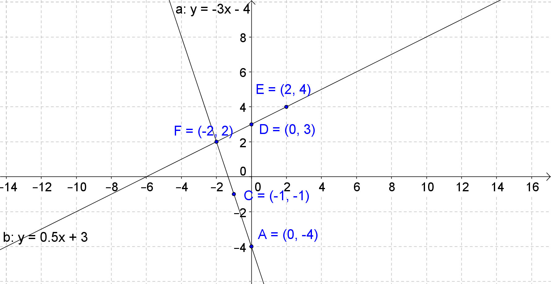


0 answers
Post by Alex Leung on August 25, 2020
At 4:02, I don't understand why the function is called a "dependent system." Is it because the points depend on the function?
1 answer
Last reply by: Ak Liu
Tue Jul 28, 2020 3:58 PM
Post by Ak Liu on July 28, 2020
On example 1, isn't the answer (1,2)? because I did the math, and the y-intercept is 1... But in your graph, it's -1.