


Professor Murray
Parametric Curves
Slide Duration:Table of Contents
Section 1: Advanced Integration Techniques
Integration by Parts
24m 52s
- Intro0:00
- Important Equation0:07
- Where It Comes From (Product Rule)0:20
- Why Use It?0:35
- Lecture Example 11:24
- Lecture Example 23:30
- Shortcut: Tabular Integration7:34
- Example7:52
- Lecture Example 310:00
- Mnemonic: LIATE14:44
- Ln, Inverse, Algebra, Trigonometry, e15:38
- Additional Example 4-1
- Additional Example 5-2
Integration of Trigonometric Functions
25m 30s
- Intro0:00
- Important Equation0:07
- Powers (Odd and Even)0:19
- What To Do1:03
- Lecture Example 11:37
- Lecture Example 23:12
- Half-Angle Formulas6:16
- Both Powers Even6:31
- Lecture Example 37:06
- Lecture Example 410:59
- Additional Example 5-1
- Additional Example 6-2
Trigonometric Substitutions
30m 9s
- Intro0:00
- Important Equations0:06
- How They Work0:35
- Example1:45
- Remember: du and dx2:50
- Lecture Example 13:43
- Lecture Example 210:01
- Lecture Example 312:04
- Additional Example 4-1
- Additional Example 5-2
Partial Fractions
41m 22s
- Intro0:00
- Overview0:07
- Why Use It?0:18
- Lecture Example 11:21
- Lecture Example 26:52
- Lecture Example 313:28
- Additional Example 4-1
- Additional Example 5-2
Integration Tables
20m
- Intro0:00
- Using Tables0:09
- Match Exactly0:32
- Lecture Example 11:16
- Lecture Example 25:28
- Lecture Example 38:51
- Additional Example 4-1
- Additional Example 5-2
Trapezoidal Rule, Midpoint Rule, Left/Right Endpoint Rule
22m 36s
- Intro0:00
- Trapezoidal Rule0:13
- Graphical Representation0:20
- How They Work1:08
- Formula1:47
- Why a Trapezoid?2:53
- Lecture Example 15:10
- Midpoint Rule8:23
- Why Midpoints?8:56
- Formula9:37
- Lecture Example 211:22
- Left/Right Endpoint Rule13:54
- Left Endpoint14:08
- Right Endpoint14:39
- Lecture Example 315:32
- Additional Example 4-1
- Additional Example 5-2
Simpson's Rule
21m 8s
- Intro0:00
- Important Equation0:03
- Estimating Area0:28
- Difference from Previous Methods0:50
- General Principle1:09
- Lecture Example 13:49
- Lecture Example 26:32
- Lecture Example 39:07
- Additional Example 4-1
- Additional Example 5-2
Improper Integration
44m 18s
- Intro0:00
- Horizontal and Vertical Asymptotes0:04
- Example: Horizontal0:16
- Formal Notation0:37
- Example: Vertical1:58
- Formal Notation2:29
- Lecture Example 15:01
- Lecture Example 27:41
- Lecture Example 311:32
- Lecture Example 415:49
- Formulas to Remember18:26
- Improper Integrals18:36
- Lecture Example 521:34
- Lecture Example 6 (Hidden Discontinuities)26:51
- Additional Example 7-1
- Additional Example 8-2
Section 2: Applications of Integrals, part 2
Arclength
23m 20s
- Intro0:00
- Important Equation0:04
- Why It Works0:49
- Common Mistake1:21
- Lecture Example 12:14
- Lecture Example 26:26
- Lecture Example 310:49
- Additional Example 4-1
- Additional Example 5-2
Surface Area of Revolution
28m 53s
- Intro0:00
- Important Equation0:05
- Surface Area0:38
- Relation to Arclength1:11
- Lecture Example 11:46
- Lecture Example 24:29
- Lecture Example 39:34
- Additional Example 4-1
- Additional Example 5-2
Hydrostatic Pressure
24m 37s
- Intro0:00
- Important Equation0:09
- Main Idea0:12
- Different Forces0:45
- Weight Density Constant1:10
- Variables (Depth and Width)2:21
- Lecture Example 13:28
- Additional Example 2-1
- Additional Example 3-2
Center of Mass
25m 39s
- Intro0:00
- Important Equation0:07
- Main Idea0:25
- Centroid1:00
- Area1:28
- Lecture Example 11:44
- Lecture Example 26:13
- Lecture Example 310:04
- Additional Example 4-1
- Additional Example 5-2
Section 3: Parametric Functions
Parametric Curves
22m 26s
- Intro0:00
- Important Equations0:05
- Slope of Tangent Line0:30
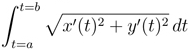
- Arc length1:03
- Lecture Example 11:40
- Lecture Example 24:23
- Lecture Example 38:38
- Additional Example 4-1
- Additional Example 5-2
Polar Coordinates
30m 59s
- Intro0:00
- Important Equations0:05
- Polar Coordinates in Calculus0:42
- Area0:58
- Arc length1:41
- Lecture Example 12:14
- Lecture Example 24:12
- Lecture Example 310:06
- Additional Example 4-1
- Additional Example 5-2
Section 4: Sequences and Series
Sequences
31m 13s
- Intro0:00
- Definition and Theorem0:05
- Monotonically Increasing0:25
- Monotonically Decreasing0:40
- Monotonic0:48
- Bounded1:00
- Theorem1:11
- Lecture Example 11:31
- Lecture Example 211:06
- Lecture Example 314:03
- Additional Example 4-1
- Additional Example 5-2
Series
31m 46s
- Intro0:00
- Important Definitions0:05
- Sigma Notation0:13
- Sequence of Partial Sums0:30
- Converging to a Limit1:49
- Diverging to Infinite2:20
- Geometric Series2:40
- Common Ratio2:47
- Sum of a Geometric Series3:09
- Test for Divergence5:11
- Not for Convergence6:06
- Lecture Example 18:32
- Lecture Example 210:25
- Lecture Example 316:26
- Additional Example 4-1
- Additional Example 5-2
Integral Test
23m 26s
- Intro0:00
- Important Theorem and Definition0:05
- Three Conditions0:25
- Converging and Diverging0:51
- P-Series1:11
- Lecture Example 12:19
- Lecture Example 25:08
- Lecture Example 36:38
- Additional Example 4-1
- Additional Example 5-2
Comparison Test
22m 44s
- Intro0:00
- Important Tests0:01
- Comparison Test0:22
- Limit Comparison Test1:05
- Lecture Example 11:44
- Lecture Example 23:52
- Lecture Example 36:01
- Lecture Example 410:04
- Additional Example 5-1
- Additional Example 6-2
Alternating Series
25m 26s
- Intro0:00
- Main Theorems0:05
- Alternation Series Test (Leibniz)0:11
- How It Works0:26
- Two Conditions0:46
- Never Use for Divergence1:12
- Estimates of Sums1:50
- Lecture Example 13:19
- Lecture Example 24:46
- Lecture Example 36:28
- Additional Example 4-1
- Additional Example 5-2
Ratio Test and Root Test
33m 27s
- Intro0:00
- Theorems and Definitions0:06
- Two Common Questions0:17
- Absolutely Convergent0:45
- Conditionally Convergent1:18
- Divergent1:51
- Missing Case2:02
- Ratio Test3:07
- Root Test4:45
- Lecture Example 15:46
- Lecture Example 29:23
- Lecture Example 313:13
- Additional Example 4-1
- Additional Example 5-2
Power Series
38m 36s
- Intro0:00
- Main Definitions and Pattern0:07
- What Is The Point0:22
- Radius of Convergence Pattern0:45
- Interval of Convergence2:42
- Lecture Example 13:24
- Lecture Example 210:55
- Lecture Example 314:44
- Additional Example 4-1
- Additional Example 5-2
Section 5: Taylor and Maclaurin Series
Taylor Series and Maclaurin Series
30m 18s
- Intro0:00
- Taylor and Maclaurin Series0:08
- Taylor Series0:12
- Maclaurin Series0:59
- Taylor Polynomial1:20
- Lecture Example 12:35
- Lecture Example 26:51
- Lecture Example 311:38
- Lecture Example 417:29
- Additional Example 5-1
- Additional Example 6-2
Taylor Polynomial Applications
50m 50s
- Intro0:00
- Main Formulas0:06
- Alternating Series Error Bound0:28
- Taylor's Remainder Theorem1:18
- Lecture Example 13:09
- Lecture Example 29:08
- Lecture Example 317:35
- Additional Example 4-1
- Additional Example 5-2
Loading...
This is a quick preview of the lesson. For full access, please Log In or Sign up.
For more information, please see full course syllabus of College Calculus: Level II
For more information, please see full course syllabus of College Calculus: Level II
Share this knowledge with your friends!

Copy & Paste this embed code into your website’s HTML
Please ensure that your website editor is in text mode when you paste the code.(In Wordpress, the mode button is on the top right corner.)
×
Since this lesson is not free, only the preview will appear on your website.
- - Allow users to view the embedded video in full-size.
 Answer Engine
 reduces to
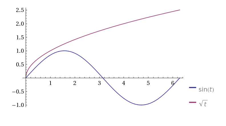


1 answer
Fri Dec 15, 2017 12:31 PM
Post by Chris DesRochers on December 11, 2017
The links to the additional problems are not working. They link to the same lecture problems and not any additional problems. :(
Thanks for your help!
1 answer
Thu Nov 20, 2014 3:20 PM
Post by David Llewellyn on November 19, 2014
How do the table and the graph in the answer to the practice question relate to the actual question? Shouldn't the graph show the relationship between x and y and not the two relationships between x (albeit a different function than in the question) and y and t?
1 answer
Fri Aug 16, 2013 6:21 PM
Post by Timothy Davis on August 14, 2013
Hi Dr. Murray,
Thanks for answering my last question. I thoroughly enjoy your videos. You mentioned that once we find the tangent line, we can use the point slope formula to find the equation of the tangent line. My question is, if we have the slope of the tangent line already defined by dy/dt / dx /dt, why do we need to find the equation of the tangent line? What is the difference between the slope of the tangent line and the equation of the tangent line? You go over this around 1:15 into your lecture.
1 answer
Wed Apr 3, 2013 11:52 AM
Post by omatseye ugen on March 12, 2012
good job . but i thought this video will involve mostly multivar. calculus
1 answer
Wed Apr 3, 2013 11:48 AM
Post by Allison Walsh on April 6, 2011
Awesome!
6 answers
Wed Apr 3, 2013 11:46 AM
Post by Wen Geng on March 7, 2011
Dr. Murray's lectures are clear, quick and concise. Very good, unlike the Chemistry ones.