


 Carleen Eaton
 Grant Fraser
 Eric Smith

Eric Smith
Systems of Linear Equations
Slide Duration:Table of Contents
Section 1: Properties of Real Numbers
Basic Types of Numbers
30m 41s
- Intro0:00
- Objectives0:07
- Basic Types of Numbers0:36
- Natural Numbers1:02
- Whole Numbers1:29
- Integers2:04
- Rational Numbers2:38
- Irrational Numbers5:06
- Imaginary Numbers6:48
- Basic Types of Numbers Cont.8:09
- The Big Picture8:10
- Real vs. Imaginary Numbers8:30
- Rational vs. Irrational Numbers8:48
- Basic Types of Numbers Cont.10:55
- Number Line11:06
- Absolute Value11:44
- Inequalities12:39
- Example 113:16
- Example 217:30
- Example 321:56
- Example 424:27
- Example 527:48
Operations on Numbers
19m 26s
- Intro0:00
- Objectives0:06
- Operations on Numbers0:25
- Addition0:53
- Subtraction1:33
- Multiplication & Division2:19
- Exponents3:24
- Bases4:04
- Square Roots4:59
- Principle Square Roots5:09
- Perfect Squares6:32
- Simplifying and Combining Roots6:52
- Example 18:16
- Example 212:30
- Example 314:02
- Example 416:27
Order of Operations
12m 6s
- Intro0:00
- Objectives0:06
- The Order of Operations0:25
- Work Inside Parentheses0:42
- Simplify Exponents0:52
- Multiplication & Division from Left to Right0:57
- Addition & Subtraction from Left to Right1:11
- Remember PEMDAS1:21
- The Order of Operations Cont.2:27
- Example2:43
- Example 13:55
- Example 25:36
- Example 37:35
- Example 48:56
Properties of Real Numbers
18m 52s
- Intro0:00
- Objectives0:07
- The Properties of Real Numbers0:23
- Commutative Property of Addition and Multiplication0:44
- Associative Property of Addition and Multiplication1:50
- Distributive Property of Multiplication Over Addition3:20
- Division Property of Zero4:46
- Division Property of One5:23
- Multiplication Property of Zero5:56
- Multiplication Property of One6:17
- Addition Property of Zero6:29
- Why Are These Properties Important?6:53
- Example 19:16
- Example 213:04
- Example 314:30
- Example 416:57
Section 2: Linear Equations
The Vocabulary of Linear Equations
12m 22s
- Intro0:00
- Objectives0:09
- The Vocabulary of Linear Equations0:44
- Variables0:52
- Terms1:09
- Coefficients1:40
- Like Terms2:18
- Examples of Like Terms2:37
- Expressions4:01
- Equations4:26
- Linear Equations5:04
- Solutions5:55
- Example 16:16
- Example 27:16
- Example 38:45
- Example 410:20
Solving Linear Equations in One Variable
28m 52s
- Intro0:00
- Objectives0:08
- Solving Linear Equations in One Variable0:34
- Conditional Cases0:51
- Identity Cases1:09
- Contradiction Cases1:30
- Solving Linear Equations in One Variable Cont.2:00
- Addition Property of Equality2:10
- Multiplication Property of Equality2:43
- Steps to Solve Linear Equations3:14
- Example 14:22
- Example 28:21
- Example 312:32
- Example 414:19
- Example 517:25
- Example 622:17
Solving Formulas
12m 2s
- Intro0:00
- Objectives0:06
- Solving Formulas0:18
- Formulas0:26
- Use the Same Properties as Solving Linear Equations1:36
- Addition Property of Equality1:55
- Multiplication Property of Equality1:58
- Steps to Solve Formulas2:43
- Example 13:56
- Example 26:09
- Example 38:39
Applications of Linear Equations
28m 41s
- Intro0:00
- Objectives0:10
- Applications of Linear Equations0:43
- The Six-Step Method to Solving Word Problems0:55
- Common Terms3:12
- Example 15:03
- Example 29:40
- Example 313:48
- Example 417:58
- Example 523:28
Applications of Linear Equations, Motion & Mixtures
24m 26s
- Intro0:00
- Objectives0:21
- Motion and Mixtures0:46
- Motion Problems: Distance, Rate, and Time1:06
- Mixture Problems: Amount, Percent, and Total1:27
- The Table Method1:58
- The Beaker Method3:38
- Example 15:05
- Example 29:44
- Example 314:20
- Example 419:13
Section 3: Graphing
Rectangular Coordinate System
22m 55s
- Intro0:00
- Objectives0:11
- The Rectangular Coordinate System0:39
- The Cartesian Coordinate System0:40
- X-Axis0:54
- Y-Axis1:04
- Origin1:11
- Quadrants1:26
- Ordered Pairs2:10
- Example 12:55
- The Rectangular Coordinate System Cont.6:09
- X-Intercept6:45
- Y-Intercept6:55
- Relation of X-Values and Y-Values7:30
- Example 211:03
- Example 312:13
- Example 414:10
- Example 518:38
Slope & Graphing
27m 58s
- Intro0:00
- Objectives0:11
- Slope and Graphing0:48
- Standard Form1:14
- Example 12:24
- Slope and Graphing Cont.4:58
- Slope, m5:07
- Slope is Rise over Run6:11
- Don't Mix Up the Coordinates8:20
- Example 29:39
- Slope and Graphing Cont.14:26
- Slope-Intercept Form14:34
- Example 316:55
- Example 418:00
- Slope and Graphing Cont.19:00
- Rewriting an Equation in Slope-Intercept Form19:39
- Rewriting an Equation in Standard Form20:09
- Slopes of Vertical & Horizontal Lines20:56
- Example 522:49
- Example 624:09
- Example 725:59
- Example 826:57
Linear Equations in Two Variables
20m 36s
- Intro0:00
- Objectives0:13
- Linear Equations in Two Variables0:36
- Point-Slope Form1:07
- Substitute in the Point and the Slope2:21
- Parallel Lines: Two Lines with the Same Slope4:05
- Perpendicular Lines: Slopes are Negative Reciprocals of Each Other4:39
- Perpendicular Lines: Product of Slopes is -15:24
- Example 16:02
- Example 27:50
- Example 310:49
- Example 413:26
- Example 515:30
- Example 617:43
Section 4: Functions
Introduction to Functions
21m 24s
- Intro0:00
- Objectives0:07
- Introduction to Functions0:58
- Relations1:03
- Functions1:37
- Independent Variables2:00
- Dependent Variables2:11
- Function Notation2:21
- Function3:43
- Input and Output3:53
- Introduction to Functions Cont.4:45
- Domain4:46
- Range4:55
- Functions Represented by a Diagram6:41
- Natural Domain9:11
- Evaluating Functions12:02
- Example 113:13
- Example 215:03
- Example 316:18
- Example 419:54
Graphing Functions
16m 12s
- Intro0:00
- Objectives0:09
- Graphing Functions0:54
- Using Slope-Intercept Form1:56
- Vertical Line Test2:58
- Determining the Domain4:20
- Determining the Range5:43
- Example 16:06
- Example 27:18
- Example 38:31
- Example 411:04
Section 5: Systems of Linear Equations
Systems of Linear Equations
25m 54s
- Intro0:00
- Objectives0:13
- Systems of Linear Equations0:46
- System of Equations0:51
- System of Linear Equations1:15
- Solutions1:35
- Points as Solutions1:53
- Finding Solutions Graphically5:13
- Example 16:37
- Example 212:07
- Systems of Linear Equations Cont.17:01
- One Solution, No Solution, or Infinite Solutions17:10
- Example 318:31
- Example 422:37
Solving a System Using Substitution
20m 1s
- Intro0:00
- Objectives0:09
- Solving a System Using Substitution0:32
- Substitution Method1:24
- Substitution Example2:35
- One Solution, No Solution, or Infinite Solutions7:50
- Example 19:45
- Example 212:48
- Example 315:01
- Example 417:30
Solving a System Using Elimination
19m 40s
- Intro0:00
- Objectives0:09
- Solving a System Using Elimination0:27
- Elimination Method0:42
- Elimination Example2:01
- One Solution, No Solution, or Infinite Solutions7:05
- Example 18:53
- Example 211:46
- Example 315:37
- Example 417:45
Applications of Systems of Equations
24m 34s
- Intro0:00
- Objectives0:12
- Applications of Systems of Equations0:30
- Word Problems1:31
- Example 12:17
- Example 27:55
- Example 313:07
- Example 417:15
Section 6: Inequalities
Solving Linear Inequalities in One Variable
17m 13s
- Intro0:00
- Objectives0:08
- Solving Linear Inequalities in One Variable0:37
- Inequality Expressions0:46
- Linear Inequality Solution Notations3:40
- Inequalities3:51
- Interval Notation4:04
- Number Lines4:43
- Set Builder Notation5:24
- Use Same Techniques as Solving Equations6:59
- 'Flip' the Sign when Multiplying or Dividing by a Negative Number7:12
- 'Flip' Example7:50
- Example 18:54
- Example 211:40
- Example 314:01
Compound Inequalities
16m 13s
- Intro0:00
- Objectives0:07
- Compound Inequalities0:37
- 'And' vs. 'Or'0:44
- 'And'3:24
- 'Or'3:35
- 'And' Symbol, or Intersection3:51
- 'Or' Symbol, or Union4:13
- Inequalities4:41
- Example 16:22
- Example 29:30
- Example 311:27
- Example 413:49
Solving Equations with Absolute Values
14m 12s
- Intro0:00
- Objectives0:08
- Solve Equations with Absolute Values0:18
- Solve Equations with Absolute Values Cont.1:11
- Steps to Solving Equations with Absolute Values2:21
- Example 13:23
- Example 26:34
- Example 310:12
Inequalities with Absolute Values
17m 7s
- Intro0:00
- Objectives0:07
- Inequalities with Absolute Values0:23
- Recall…2:08
- Example 13:39
- Example 26:06
- Example 38:14
- Example 410:29
- Example 513:29
Graphing Inequalities in Two Variables
15m 33s
- Intro0:00
- Objectives0:07
- Graphing Inequalities in Two Variables0:32
- Split Graph into Two Regions1:53
- Graphing Inequalities5:44
- Test Points6:20
- Example 17:11
- Example 210:17
- Example 313:06
Systems of Inequalities
21m 13s
- Intro0:00
- Objectives0:08
- Systems of Inequalities0:24
- Test Points1:10
- Steps to Solve Systems of Inequalities1:25
- Example 12:23
- Example 27:28
- Example 312:51
Section 7: Polynomials
Integer Exponents
44m 51s
- Intro0:00
- Objectives0:09
- Integer Exponents0:42
- Exponents 'Package' Multiplication1:25
- Example 12:00
- Example 23:13
- Integer Exponents Cont.4:50
- Product Rule for Exponents4:51
- Example 37:16
- Example 410:15
- Integer Exponents Cont.13:13
- Power Rule for Exponents13:14
- Power Rule with Multiplication and Division15:33
- Example 516:18
- Integer Exponents Cont.20:04
- Example 620:41
- Integer Exponents Cont.25:52
- Zero Exponent Rule25:53
- Quotient Rule28:24
- Negative Exponents30:14
- Negative Exponent Rule32:27
- Example 734:05
- Example 836:15
- Example 939:33
- Example 1043:16
Adding & Subtracting Polynomials
18m 33s
- Intro0:00
- Objectives0:07
- Adding and Subtracting Polynomials0:25
- Terms0:33
- Coefficients0:51
- Leading Coefficients1:13
- Like Terms1:29
- Polynomials2:21
- Monomials, Binomials, Trinomials, and Polynomials5:41
- Degrees7:00
- Evaluating Polynomials8:12
- Adding and Subtracting Polynomials Cont.9:25
- Example 111:48
- Example 213:00
- Example 314:41
- Example 416:15
Multiplying Polynomials
25m 7s
- Intro0:00
- Objectives0:06
- Multiplying Polynomials0:41
- Distributive Property1:00
- Example 12:49
- Multiplying Polynomials Cont.8:22
- Organize Terms with a Table8:23
- Example 213:40
- Multiplying Polynomials Cont.16:33
- Multiplying Binomials with FOIL16:48
- Example 318:49
- Example 420:04
- Example 521:42
Dividing Polynomials
44m 56s
- Intro0:00
- Objectives0:07
- Dividing Polynomials0:29
- Dividing Polynomials by Monomials2:10
- Dividing Polynomials by Polynomials2:59
- Dividing Numbers4:09
- Dividing Polynomials Example8:39
- Example 112:35
- Example 214:40
- Example 316:45
- Example 421:13
- Example 524:33
- Example 629:02
- Dividing Polynomials with Synthetic Division Method33:36
- Example 738:43
- Example 842:24
Section 8: Factoring Polynomials
Greatest Common Factor & Factor by Grouping
28m 27s
- Intro0:00
- Objectives0:09
- Greatest Common Factor0:31
- Factoring0:40
- Greatest Common Factor (GCF)1:48
- GCF for Polynomials3:28
- Factoring Polynomials6:45
- Prime8:21
- Example 19:14
- Factor by Grouping14:30
- Steps to Factor by Grouping17:03
- Example 217:43
- Example 319:20
- Example 420:41
- Example 522:29
- Example 626:11
Factoring Trinomials
21m 44s
- Intro0:00
- Objectives0:06
- Factoring Trinomials0:25
- Recall FOIL0:26
- Factor a Trinomial by Reversing FOIL1:52
- Tips when Using Reverse FOIL5:31
- Example 17:04
- Example 29:09
- Example 311:15
- Example 413:41
- Factoring Trinomials Cont.15:50
- Example 518:42
Factoring Trinomials Using the AC Method
30m 9s
- Intro0:00
- Objectives0:08
- Factoring Trinomials Using the AC Method0:27
- Factoring when Leading Term has Coefficient Other Than 11:07
- Reversing FOIL1:18
- Example 11:46
- Example 24:28
- Factoring Trinomials Using the AC Method Cont.7:45
- The AC Method8:03
- Steps to Using the AC Method8:19
- Tips on Using the AC Method9:29
- Example 310:45
- Example 416:50
- Example 521:08
- Example 624:58
Special Factoring Techniques
30m 14s
- Intro0:00
- Objectives0:07
- Special Factoring Techniques0:26
- Difference of Squares1:46
- Perfect Square Trinomials2:38
- No Sum of Squares3:32
- Special Factoring Techniques Cont.4:03
- Difference of Squares Example4:04
- Perfect Square Trinomials Example5:29
- Example 17:31
- Example 29:59
- Example 311:47
- Example 415:09
- Special Factoring Techniques Cont.19:07
- Sum of Cubes and Difference of Cubes19:08
- Example 523:13
- Example 626:12
Section 9: Quadratic Equations
Solving Quadratic Equations by Factoring
23m 38s
- Intro0:00
- Objectives0:08
- Solving Quadratic Equations by Factoring0:19
- Quadratic Equations0:20
- Zero Factor Property1:39
- Zero Factor Property Example2:34
- Example 14:00
- Solving Quadratic Equations by Factoring Cont.5:54
- Example 27:28
- Example 311:09
- Example 414:22
- Solving Quadratic Equations by Factoring Cont.18:17
- Higher Degree Polynomial Equations18:18
- Example 520:22
Solving Quadratic Equations
29m 27s
- Intro0:00
- Objectives0:12
- Solving Quadratic Equations0:29
- Linear Factors0:38
- Not All Quadratics Factor Easily1:22
- Principle of Square Roots3:36
- Completing the Square4:50
- Steps for Using Completing the Square5:15
- Completing the Square Works on All Quadratic Equations6:41
- The Quadratic Formula7:28
- Discriminants8:25
- Solving Quadratic Equations - Summary10:11
- Example 111:54
- Example 213:03
- Example 316:30
- Example 421:29
- Example 525:07
Equations in Quadratic Form
16m 47s
- Intro0:00
- Objectives0:08
- Equations in Quadratic Form0:24
- Using a Substitution0:53
- U-Substitution1:26
- Example 12:07
- Example 25:36
- Example 38:31
- Example 411:14
Quadratic Formulas & Applications
29m 4s
- Intro0:00
- Objectives0:09
- Quadratic Formulas and Applications0:35
- Squared Variable0:40
- Principle of Square Roots0:51
- Example 11:09
- Example 22:04
- Quadratic Formulas and Applications Cont.3:34
- Example 34:42
- Example 413:33
- Example 520:50
Graphs of Quadratics
26m 53s
- Intro0:00
- Objectives0:06
- Graphs of Quadratics0:39
- Axis of Symmetry1:46
- Vertex2:12
- Transformations2:57
- Graphing in Quadratic Standard Form3:23
- Example 15:06
- Example 26:02
- Example 39:07
- Graphs of Quadratics Cont.11:26
- Completing the Square12:02
- Vertex Shortcut12:16
- Example 413:49
- Example 517:25
- Example 620:07
- Example 723:43
Polynomial Inequalities
21m 42s
- Intro0:00
- Objectives0:07
- Polynomial Inequalities0:30
- Solving Polynomial Inequalities1:20
- Example 12:45
- Polynomial Inequalities Cont.5:12
- Larger Polynomials5:13
- Positive or Negative Intervals7:16
- Example 29:01
- Example 313:53
Section 10: Rational Equations
Multiply & Divide Rational Expressions
26m 41s
- Intro0:00
- Objectives0:09
- Multiply and Divide Rational Expressions0:44
- Rational Numbers0:55
- Dividing by Zero1:45
- Canceling Extra Factors2:43
- Negative Signs in Fractions4:52
- Multiplying Fractions6:26
- Dividing Fractions7:17
- Example 18:04
- Example 214:01
- Example 316:23
- Example 418:56
- Example 522:43
Adding & Subtracting Rational Expressions
20m 24s
- Intro0:00
- Objectives0:07
- Adding and Subtracting Rational Expressions0:41
- Common Denominators0:52
- Common Denominator Examples1:14
- Steps to Adding and Subtracting Rational Expressions2:39
- Example 13:34
- Example 25:27
- Adding and Subtracting Rational Expressions Cont.6:57
- Least Common Denominators6:58
- Transitioning from Fractions to Rational Expressions9:08
- Identifying Least Common Denominators for Rational Expressions9:56
- Subtracting vs. Adding10:41
- Example 311:19
- Example 412:36
- Example 515:08
- Example 616:46
Complex Fractions
18m 23s
- Intro0:00
- Objectives0:09
- Complex Fractions0:37
- Dividing to Simplify Complex Fractions1:10
- Example 12:03
- Example 23:58
- Complex Fractions Cont.9:15
- Using the Least Common Denominator to Simplify Complex Fractions9:16
- Both Methods Lead to the Same Answer10:07
- Example 310:42
- Example 414:28
Solving Rational Equations
16m 24s
- Intro0:00
- Objectives0:07
- Solving Rational Equations0:23
- Isolate the Specified Variable1:23
- Example 11:58
- Example 25:00
- Example 38:23
- Example 413:25
Rational Inequalities
18m 54s
- Intro0:00
- Objectives0:06
- Rational Inequalities0:18
- Testing Intervals for Rational Inequalities0:38
- Steps to Solving Rational Inequalities1:05
- Tips to Solving Rational Inequalities2:27
- Example 13:33
- Example 212:21
Applications of Rational Expressions
20m 20s
- Intro0:00
- Objectives0:07
- Applications of Rational Expressions0:27
- Work Problems1:05
- Example 12:58
- Example 26:45
- Example 313:17
- Example 416:37
Variation & Proportion
27m 4s
- Intro0:00
- Objectives0:10
- Variation and Proportion0:34
- Variation0:35
- Inverse Variation1:01
- Direct Variation1:10
- Setting Up Proportions1:31
- Example 12:27
- Example 25:36
- Variation and Proportion Cont.8:29
- Inverse Variation8:30
- Example 39:20
- Variation and Proportion Cont.12:41
- Constant of Proportionality12:42
- Example 413:59
- Variation and Proportion Cont.16:17
- Varies Directly as the nth Power16:30
- Varies Inversely as the nth Power16:53
- Varies Jointly17:09
- Combining Variation Models17:36
- Example 519:09
- Example 622:10
Section 11: Radical Equations
Rational Exponents
14m 32s
- Intro0:00
- Objectives0:07
- Rational Exponents0:32
- Power on Top, Root on Bottom1:05
- Example 11:37
- Rational Exponents Cont.4:04
- Using Rules from Exponents for Radicals as Exponents4:05
- Combining Terms Under a Single Root4:50
- Example 25:21
- Example 37:39
- Example 411:23
- Example 513:14
Simplify Rational Exponents
15m 12s
- Intro0:00
- Objectives0:07
- Simplify Rational Exponents0:25
- Product Rule for Radicals0:26
- Product Rule to Simplify Square Roots1:11
- Quotient Rule for Radicals1:42
- Applications of Product and Quotient Rules2:17
- Higher Roots2:48
- Example 13:39
- Example 26:35
- Example 38:41
- Example 411:09
Adding & Subtracting Radicals
17m 22s
- Intro0:00
- Objectives0:07
- Adding and Subtracting Radicals0:33
- Like Terms1:29
- Bases and Exponents May be Different2:02
- Bases and Powers Must be Same when Adding and Subtracting2:42
- Add Radicals' Coefficients3:55
- Example 14:47
- Example 26:00
- Adding and Subtracting Radicals Cont.7:10
- Simplify the Bases to Look the Same7:25
- Example 38:23
- Example 411:45
- Example 515:10
Multiply & Divide Radicals
19m 24s
- Intro0:00
- Objectives0:08
- Multiply and Divide Radicals0:25
- Rules for Working With Radicals0:26
- Using FOIL for Radicals1:11
- Don’t Distribute Powers2:54
- Dividing Radical Expressions4:25
- Rationalizing Denominators6:40
- Example 17:22
- Example 28:32
- Multiply and Divide Radicals Cont.9:23
- Rationalizing Denominators with Higher Roots9:25
- Example 310:51
- Example 411:53
- Multiply and Divide Radicals Cont.13:13
- Rationalizing Denominators with Conjugates13:14
- Example 515:52
- Example 617:25
Solving Radical Equations
15m 5s
- Intro0:00
- Objectives0:07
- Solving Radical Equations0:17
- Radical Equations0:18
- Isolate the Roots and Raise to Power0:34
- Example 11:13
- Example 23:09
- Solving Radical Equations Cont.7:04
- Solving Radical Equations with More than One Radical7:05
- Example 37:54
- Example 413:07
Complex Numbers
29m 16s
- Intro0:00
- Objectives0:06
- Complex Numbers1:05
- Imaginary Numbers1:08
- Complex Numbers2:27
- Real Parts2:48
- Imaginary Parts2:51
- Commutative, Associative, and Distributive Properties3:35
- Adding and Subtracting Complex Numbers4:04
- Multiplying Complex Numbers6:16
- Dividing Complex Numbers8:59
- Complex Conjugate9:07
- Simplifying Powers of i14:34
- Shortcut for Simplifying Powers of i18:33
- Example 121:14
- Example 222:15
- Example 323:38
- Example 426:33
Loading...
This is a quick preview of the lesson. For full access, please Log In or Sign up.
For more information, please see full course syllabus of Algebra 1
For more information, please see full course syllabus of Algebra 1
Share this knowledge with your friends!

Copy & Paste this embed code into your website’s HTML
Please ensure that your website editor is in text mode when you paste the code.(In Wordpress, the mode button is on the top right corner.)
×
Since this lesson is not free, only the preview will appear on your website.
- - Allow users to view the embedded video in full-size.
 Answer Engine
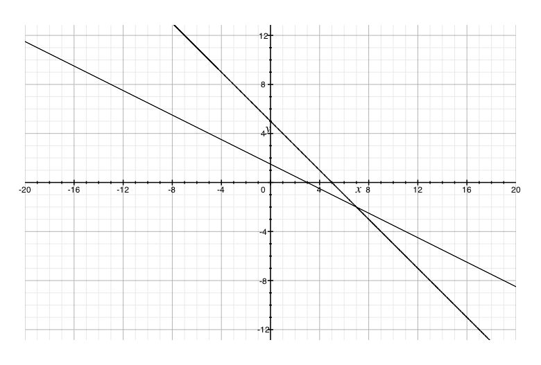


0 answers
Post by Rose A on February 19, 2018
Some of the practice questions are wrong...
It's not you that does the pracice questions from what I understood?... who can I contact for issues with the practice questions!?
1 answer
Thu Dec 31, 2015 6:32 PM
Post by Bongani Makhathini on December 30, 2015
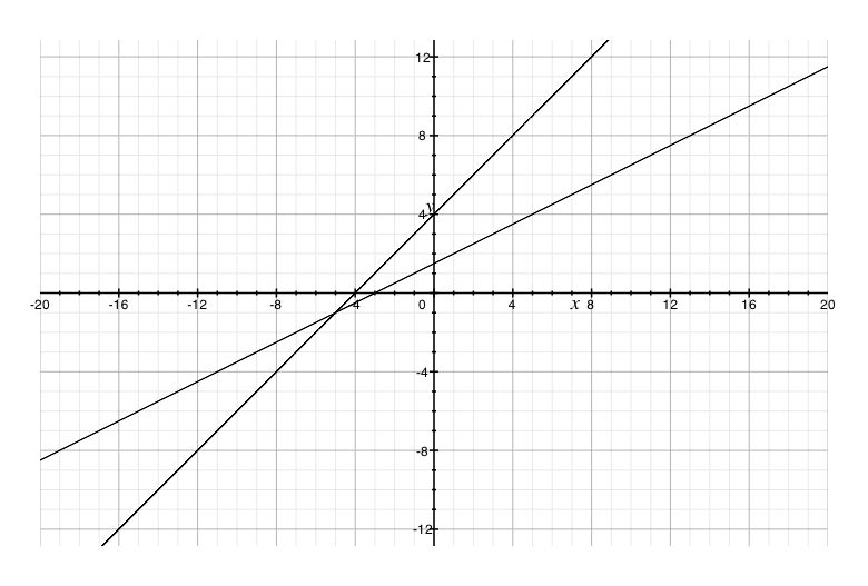
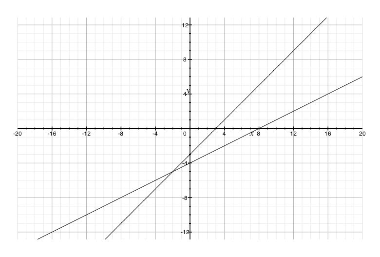
I believe that example 3 does have a solution, its just that the lines will across outside the graphing paper displayed on the screen as the lines progress. I came to this conclusion because the points 4, 2 and 6 are even numbers. However, 3 is an odd number, tilting the line just slightly anti-clockwise. :-)
0 answers
Post by Farhat Muruwat on March 24, 2014
Step 3. 2y − x = 3 → ( 0,[3/2] ),( − [3/2],0 )
How did you get 2y - x = 3?
0 answers
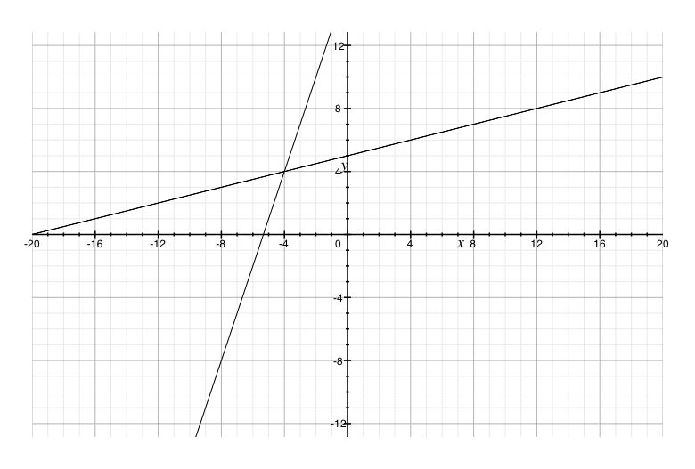
Post by Farhat Muruwat on March 24, 2014
Q. Solving the system by graphing
y − x = 42y − x = 3
Step 1. Find two points for each equation by setting x = 0 then y = 0
Step 2. y − x = 4 → ( 0,4 ),( − 4,0 )
How did you get y - x = 4?