


Raffi Hovasapian
Functions of Several Variable
Slide Duration:Table of Contents
Section 1: Vectors
Points & Vectors
28m 23s
- Intro0:00
- Points and Vectors1:02
- A Point in a Plane1:03
- A Point in Space3:14
- Notation for a Space of a Given Space6:34
- Introduction to Vectors9:51
- Adding Vectors14:51
- Example 116:52
- Properties of Vector Addition18:24
- Example 221:01
- Two More Properties of Vector Addition24:16
- Multiplication of a Vector by a Constant25:27
Scalar Product & Norm
30m 25s
- Intro0:00
- Scalar Product and Norm1:05
- Introduction to Scalar Product1:06
- Example 13:21
- Properties of Scalar Product6:14
- Definition: Orthogonal11:41
- Example 2: Orthogonal14:19
- Definition: Norm of a Vector15:30
- Example 319:37
- Distance Between Two Vectors22:05
- Example 427:19
More on Vectors & Norms
38m 18s
- Intro0:00
- More on Vectors and Norms0:38
- Open Disc0:39
- Close Disc3:14
- Open Ball, Closed Ball, and the Sphere5:22
- Property and Definition of Unit Vector7:16
- Example 114:04
- Three Special Unit Vectors17:24
- General Pythagorean Theorem19:44
- Projection23:00
- Example 228:35
- Example 335:54
Inequalities & Parametric Lines
33m 19s
- Intro0:00
- Inequalities and Parametric Lines0:30
- Starting Example0:31
- Theorem 15:10
- Theorem 27:22
- Definition 1: Parametric Equation of a Straight Line10:16
- Definition 217:38
- Example 121:19
- Example 225:20
Planes
29m 59s
- Intro0:00
- Planes0:18
- Definition 10:19
- Example 17:04
- Example 212:45
- General Definitions and Properties: 2 Vectors are Said to Be Paralleled If14:50
- Example 316:44
- Example 420:17
More on Planes
34m 18s
- Intro0:00
- More on Planes0:25
- Example 10:26
- Distance From Some Point in Space to a Given Plane: Derivation10:12
- Final Formula for Distance21:20
- Example 223:09
- Example 3: Part 126:56
- Example 3: Part 231:46
Section 2: Differentiation of Vectors
Maps, Curves & Parameterizations
29m 48s
- Intro0:00
- Maps, Curves and Parameterizations1:10
- Recall1:11
- Looking at y = x2 or f(x) = x22:23
- Departure Space & Arrival Space7:01
- Looking at a 'Function' from ℝ to ℝ210:36
- Example 114:50
- Definition 1: Parameterized Curve17:33
- Example 221:56
- Example 325:16
Differentiation of Vectors
39m 40s
- Intro0:00
- Differentiation of Vectors0:18
- Example 10:19
- Definition 1: Velocity of a Curve1:45
- Line Tangent to a Curve6:10
- Example 27:40
- Definition 2: Speed of a Curve12:18
- Example 313:53
- Definition 3: Acceleration Vector16:37
- Two Definitions for the Scalar Part of Acceleration17:22
- Rules for Differentiating Vectors: 119:52
- Rules for Differentiating Vectors: 221:28
- Rules for Differentiating Vectors: 322:03
- Rules for Differentiating Vectors: 424:14
- Example 426:57
Section 3: Functions of Several Variables
Functions of Several Variable
29m 31s
- Intro0:00
- Length of a Curve in Space0:25
- Definition 1: Length of a Curve in Space0:26
- Extended Form2:06
- Example 13:40
- Example 26:28
- Functions of Several Variable8:55
- Functions of Several Variable8:56
- General Examples11:11
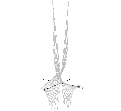
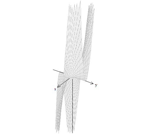
- Graph by Plotting13:00
- Example 116:31
- Definition 118:33
- Example 222:15
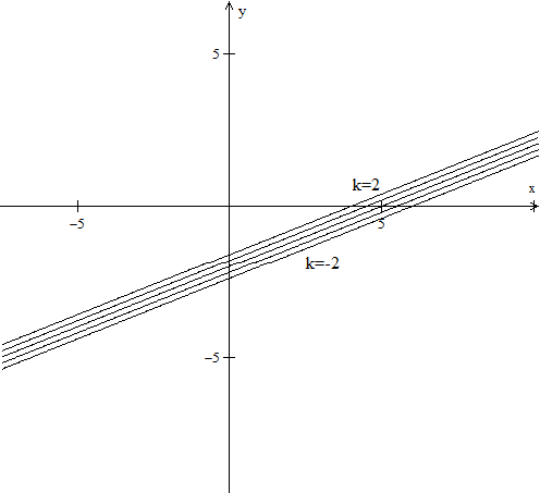
- Equipotential Surfaces25:27
- Isothermal Surfaces27:30
Partial Derivatives
23m 31s
- Intro0:00
- Partial Derivatives0:19
- Example 10:20
- Example 25:30
- Example 37:48
- Example 49:19
- Definition 112:19
- Example 514:24
- Example 616:14
- Notation and Properties for Gradient20:26
Higher and Mixed Partial Derivatives
30m 48s
- Intro0:00
- Higher and Mixed Partial Derivatives0:45
- Definition 1: Open Set0:46
- Notation: Partial Derivatives5:39
- Example 112:00
- Theorem 114:25
- Now Consider a Function of Three Variables16:50
- Example 220:09
- Caution23:16
- Example 325:42
Section 4: Chain Rule and The Gradient
The Chain Rule
28m 3s
- Intro0:00
- The Chain Rule0:45
- Conceptual Example0:46
- Example 15:10
- The Chain Rule10:11
- Example 2: Part 119:06
- Example 2: Part 2 - Solving Directly25:26
Tangent Plane
42m 25s
- Intro0:00
- Tangent Plane1:02
- Tangent Plane Part 11:03
- Tangent Plane Part 210:00
- Tangent Plane Part 318:18
- Tangent Plane Part 421:18
- Definition 1: Tangent Plane to a Surface27:46
- Example 1: Find the Equation of the Plane Tangent to the Surface31:18
- Example 2: Find the Tangent Line to the Curve36:54
Further Examples with Gradients & Tangents
47m 11s
- Intro0:00
- Example 1: Parametric Equation for the Line Tangent to the Curve of Two Intersecting Surfaces0:41
- Part 1: Question0:42
- Part 2: When Two Surfaces in ℝ3 Intersect4:31
- Part 3: Diagrams7:36
- Part 4: Solution12:10
- Part 5: Diagram of Final Answer23:52
- Example 2: Gradients & Composite Functions26:42
- Part 1: Question26:43
- Part 2: Solution29:21
- Example 3: Cos of the Angle Between the Surfaces39:20
- Part 1: Question39:21
- Part 2: Definition of Angle Between Two Surfaces41:04
- Part 3: Solution42:39
Directional Derivative
41m 22s
- Intro0:00
- Directional Derivative0:10
- Rate of Change & Direction Overview0:11
- Rate of Change : Function of Two Variables4:32
- Directional Derivative10:13
- Example 118:26
- Examining Gradient of f(p) ∙ A When A is a Unit Vector25:30
- Directional Derivative of f(p)31:03
- Norm of the Gradient f(p)33:23
- Example 234:53
A Unified View of Derivatives for Mappings
39m 41s
- Intro0:00
- A Unified View of Derivatives for Mappings1:29
- Derivatives for Mappings1:30
- Example 15:46
- Example 28:25
- Example 312:08
- Example 414:35
- Derivative for Mappings of Composite Function17:47
- Example 522:15
- Example 628:42
Section 5: Maxima and Minima
Maxima & Minima
36m 41s
- Intro0:00
- Maxima and Minima0:35
- Definition 1: Critical Point0:36
- Example 1: Find the Critical Values2:48
- Definition 2: Local Max & Local Min10:03
- Theorem 114:10
- Example 2: Local Max, Min, and Extreme18:28
- Definition 3: Boundary Point27:00
- Definition 4: Closed Set29:50
- Definition 5: Bounded Set31:32
- Theorem 233:34
Further Examples with Extrema
32m 48s
- Intro0:00
- Further Example with Extrema1:02
- Example 1: Max and Min Values of f on the Square1:03
- Example 2: Find the Extreme for f(x,y) = x² + 2y² - x10:44
- Example 3: Max and Min Value of f(x,y) = (x²+ y²)⁻¹ in the Region (x -2)²+ y² ≤ 117:20
Lagrange Multipliers
32m 32s
- Intro0:00
- Lagrange Multipliers1:13
- Theorem 11:14
- Method6:35
- Example 1: Find the Largest and Smallest Values that f Achieves Subject to g9:14
- Example 2: Find the Max & Min Values of f(x,y)= 3x + 4y on the Circle x² + y² = 122:18
More Lagrange Multiplier Examples
27m 42s
- Intro0:00
- Example 1: Find the Point on the Surface z² -xy = 1 Closet to the Origin0:54
- Part 10:55
- Part 27:37
- Part 310:44
- Example 2: Find the Max & Min of f(x,y) = x² + 2y - x on the Closed Disc of Radius 1 Centered at the Origin16:05
- Part 116:06
- Part 219:33
- Part 323:17
Lagrange Multipliers, Continued
31m 47s
- Intro0:00
- Lagrange Multipliers0:42
- First Example of Lesson 200:44
- Let's Look at This Geometrically3:12
- Example 1: Lagrange Multiplier Problem with 2 Constraints8:42
- Part 1: Question8:43
- Part 2: What We Have to Solve15:13
- Part 3: Case 120:49
- Part 4: Case 222:59
- Part 5: Final Solution25:45
Section 6: Line Integrals and Potential Functions
Line Integrals
36m 8s
- Intro0:00
- Line Integrals0:18
- Introduction to Line Integrals0:19
- Definition 1: Vector Field3:57
- Example 15:46
- Example 2: Gradient Operator & Vector Field8:06
- Example 312:19
- Vector Field, Curve in Space & Line Integrals14:07
- Definition 2: F(C(t)) ∙ C'(t) is a Function of t17:45
- Example 418:10
- Definition 3: Line Integrals20:21
- Example 525:00
- Example 630:33
More on Line Integrals
28m 4s
- Intro0:00
- More on Line Integrals0:10
- Line Integrals Notation0:11
- Curve Given in Non-parameterized Way: In General4:34
- Curve Given in Non-parameterized Way: For the Circle of Radius r6:07
- Curve Given in Non-parameterized Way: For a Straight Line Segment Between P & Q6:32
- The Integral is Independent of the Parameterization Chosen7:17
- Example 1: Find the Integral on the Ellipse Centered at the Origin9:18
- Example 2: Find the Integral of the Vector Field16:26
- Discussion of Result and Vector Field for Example 223:52
- Graphical Example26:03
Line Integrals, Part 3
29m 30s
- Intro0:00
- Line Integrals0:12
- Piecewise Continuous Path0:13
- Closed Path1:47
- Example 1: Find the Integral3:50
- The Reverse Path14:14
- Theorem 116:18
- Parameterization for the Reverse Path17:24
- Example 218:50
- Line Integrals of Functions on ℝn21:36
- Example 324:20
Potential Functions
40m 19s
- Intro0:00
- Potential Functions0:08
- Definition 1: Potential Functions0:09
- Definition 2: An Open Set S is Called Connected if…5:52
- Theorem 18:19
- Existence of a Potential Function11:04
- Theorem 218:06
- Example 122:18
- Contrapositive and Positive Form of the Theorem28:02
- The Converse is Not Generally True30:59
- Our Theorem32:55
- Compare the n-th Term Test for Divergence of an Infinite Series36:00
- So for Our Theorem38:16
Potential Functions, Continued
31m 45s
- Intro0:00
- Potential Functions0:52
- Theorem 10:53
- Example 14:00
- Theorem in 3-Space14:07
- Example 217:53
- Example 324:07
Potential Functions, Conclusion & Summary
28m 22s
- Intro0:00
- Potential Functions0:16
- Theorem 10:17
- In Other Words3:25
- Corollary5:22
- Example 17:45
- Theorem 211:34
- Summary on Potential Functions 115:32
- Summary on Potential Functions 217:26
- Summary on Potential Functions 318:43
- Case 119:24
- Case 220:48
- Case 321:35
- Example 223:59
Section 7: Double Integrals
Double Integrals
29m 46s
- Intro0:00
- Double Integrals0:52
- Introduction to Double Integrals0:53
- Function with Two Variables3:39
- Example 1: Find the Integral of xy³ over the Region x ϵ[1,2] & y ϵ[4,6]9:42
- Example 2: f(x,y) = x²y & R be the Region Such That x ϵ[2,3] & x² ≤ y ≤ x³15:07
- Example 3: f(x,y) = 4xy over the Region Bounded by y= 0, y= x, and y= -x+319:20
Polar Coordinates
36m 17s
- Intro0:00
- Polar Coordinates0:50
- Polar Coordinates0:51
- Example 1: Let (x,y) = (6,√6), Convert to Polar Coordinates3:24
- Example 2: Express the Circle (x-2)² + y² = 4 in Polar Form.5:46
- Graphing Function in Polar Form.10:02
- Converting a Region in the xy-plane to Polar Coordinates14:14
- Example 3: Find the Integral over the Region Bounded by the Semicircle20:06
- Example 4: Find the Integral over the Region27:57
- Example 5: Find the Integral of f(x,y) = x² over the Region Contained by r= 1 - cosθ32:55
Green's Theorem
38m 1s
- Intro0:00
- Green's Theorem0:38
- Introduction to Green's Theorem and Notations0:39
- Green's Theorem3:17
- Example 1: Find the Integral of the Vector Field around the Ellipse8:30
- Verifying Green's Theorem with Example 115:35
- A More General Version of Green's Theorem20:03
- Example 222:59
- Example 326:30
- Example 432:05
Divergence & Curl of a Vector Field
37m 16s
- Intro0:00
- Divergence & Curl of a Vector Field0:18
- Definitions: Divergence(F) & Curl(F)0:19
- Example 1: Evaluate Divergence(F) and Curl(F)3:43
- Properties of Divergence9:24
- Properties of Curl12:24
- Two Versions of Green's Theorem: Circulation - Curl17:46
- Two Versions of Green's Theorem: Flux Divergence19:09
- Circulation-Curl Part 120:08
- Circulation-Curl Part 228:29
- Example 232:06
Divergence & Curl, Continued
33m 7s
- Intro0:00
- Divergence & Curl, Continued0:24
- Divergence Part 10:25
- Divergence Part 2: Right Normal Vector and Left Normal Vector5:28
- Divergence Part 39:09
- Divergence Part 413:51
- Divergence Part 519:19
- Example 123:40
Final Comments on Divergence & Curl
16m 49s
- Intro0:00
- Final Comments on Divergence and Curl0:37
- Several Symbolic Representations for Green's Theorem0:38
- Circulation-Curl9:44
- Flux Divergence11:02
- Closing Comments on Divergence and Curl15:04
Section 8: Triple Integrals
Triple Integrals
27m 24s
- Intro0:00
- Triple Integrals0:21
- Example 12:01
- Example 29:42
- Example 315:25
- Example 420:54
Cylindrical & Spherical Coordinates
35m 33s
- Intro0:00
- Cylindrical and Spherical Coordinates0:42
- Cylindrical Coordinates0:43
- When Integrating Over a Region in 3-space, Upon Transformation the Triple Integral Becomes..4:29
- Example 16:27
- The Cartesian Integral15:00
- Introduction to Spherical Coordinates19:44
- Reason It's Called Spherical Coordinates22:49
- Spherical Transformation26:12
- Example 229:23
Section 9: Surface Integrals and Stokes' Theorem
Parameterizing Surfaces & Cross Product
41m 29s
- Intro0:00
- Parameterizing Surfaces0:40
- Describing a Line or a Curve Parametrically0:41
- Describing a Line or a Curve Parametrically: Example1:52
- Describing a Surface Parametrically2:58
- Describing a Surface Parametrically: Example5:30
- Recall: Parameterizations are not Unique7:18
- Example 1: Sphere of Radius R8:22
- Example 2: Another P for the Sphere of Radius R10:52
- This is True in General13:35
- Example 3: Paraboloid15:05
- Example 4: A Surface of Revolution around z-axis18:10
- Cross Product23:15
- Defining Cross Product23:16
- Example 5: Part 128:04
- Example 5: Part 2 - Right Hand Rule32:31
- Example 637:20
Tangent Plane & Normal Vector to a Surface
37m 6s
- Intro0:00
- Tangent Plane and Normal Vector to a Surface0:35
- Tangent Plane and Normal Vector to a Surface Part 10:36
- Tangent Plane and Normal Vector to a Surface Part 25:22
- Tangent Plane and Normal Vector to a Surface Part 313:42
- Example 1: Question & Solution17:59
- Example 1: Illustrative Explanation of the Solution28:37
- Example 2: Question & Solution30:55
- Example 2: Illustrative Explanation of the Solution35:10
Surface Area
32m 48s
- Intro0:00
- Surface Area0:27
- Introduction to Surface Area0:28
- Given a Surface in 3-space and a Parameterization P3:31
- Defining Surface Area7:46
- Curve Length10:52
- Example 1: Find the Are of a Sphere of Radius R15:03
- Example 2: Find the Area of the Paraboloid z= x² + y² for 0 ≤ z ≤ 519:10
- Example 2: Writing the Answer in Polar Coordinates28:07
Surface Integrals
46m 52s
- Intro0:00
- Surface Integrals0:25
- Introduction to Surface Integrals0:26
- General Integral for Surface Are of Any Parameterization3:03
- Integral of a Function Over a Surface4:47
- Example 19:53
- Integral of a Vector Field Over a Surface17:20
- Example 222:15
- Side Note: Be Very Careful28:58
- Example 330:42
- Summary43:57
Divergence & Curl in 3-Space
23m 40s
- Intro0:00
- Divergence and Curl in 3-Space0:26
- Introduction to Divergence and Curl in 3-Space0:27
- Define: Divergence of F2:50
- Define: Curl of F4:12
- The Del Operator6:25
- Symbolically: Div(F)9:03
- Symbolically: Curl(F)10:50
- Example 114:07
- Example 218:01
Divergence Theorem in 3-Space
34m 12s
- Intro0:00
- Divergence Theorem in 3-Space0:36
- Green's Flux-Divergence0:37
- Divergence Theorem in 3-Space3:34
- Note: Closed Surface6:43
- Figure: Paraboloid8:44
- Example 112:13
- Example 218:50
- Recap for Surfaces: Introduction27:50
- Recap for Surfaces: Surface Area29:16
- Recap for Surfaces: Surface Integral of a Function29:50
- Recap for Surfaces: Surface Integral of a Vector Field30:39
- Recap for Surfaces: Divergence Theorem32:32
Stokes' Theorem, Part 1
22m 1s
- Intro0:00
- Stokes' Theorem0:25
- Recall Circulation-Curl Version of Green's Theorem0:26
- Constructing a Surface in 3-Space2:26
- Stokes' Theorem5:34
- Note on Curve and Vector Field in 3-Space9:50
- Example 1: Find the Circulation of F around the Curve12:40
- Part 1: Question12:48
- Part 2: Drawing the Figure13:56
- Part 3: Solution16:08
Stokes' Theorem, Part 2
20m 32s
- Intro0:00
- Example 1: Calculate the Boundary of the Surface and the Circulation of F around this Boundary0:30
- Part 1: Question0:31
- Part 2: Drawing the Figure2:02
- Part 3: Solution5:24
- Example 2: Calculate the Boundary of the Surface and the Circulation of F around this Boundary13:11
- Part 1: Question13:12
- Part 2: Solution13:56
Loading...
This is a quick preview of the lesson. For full access, please Log In or Sign up.
For more information, please see full course syllabus of Multivariable Calculus
For more information, please see full course syllabus of Multivariable Calculus
Share this knowledge with your friends!

Copy & Paste this embed code into your website’s HTML
Please ensure that your website editor is in text mode when you paste the code.(In Wordpress, the mode button is on the top right corner.)
×
Since this lesson is not free, only the preview will appear on your website.
- - Allow users to view the embedded video in full-size.
 Answer Engine
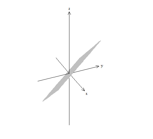


1 answer
Thu Aug 14, 2014 12:49 AM
Post by Denny Yang on August 13, 2014
One thing that annoys me in this lecture is that you keep forgetting to put the vectors arrows on top of the velocity functions and the c(t). I do not know which one is the vector and which one is not if you dont put the arrows. Just my way of understanding it better..
2 answers
Last reply by: George Chumbipuma
Wed Feb 3, 2016 7:39 AM
Post by Alex Emil on February 3, 2014
I love these lectures, they are awesome. I was wondering if it was possible for you to do a short course on using Maple for doing stuff in calculus 3 and diff equns? Thank you professor!!
2 answers
Last reply by: Laney M
Thu Jan 23, 2014 11:46 PM
Post by Laney M on January 22, 2014
Hi Raffi,
In your example 1, you used x and y variables to the 2nd degree. What if f(x,y)= x and y with different degrees. For example, f(x,y)= 2x-y^2. Would you graph it the same way?
3 answers
Wed Oct 30, 2013 4:05 AM
Post by Christian Fischer on October 27, 2013
Dear Raffi, I have a specific confusion regarding bridging the gap between the original function f(x) and the vector form and I would really appreciate your help on this one:
If we have a traditional function f(x)=x^2 and we take the derivative we get f’(x)=2x which is a straight line in the Cartesian coordinate system. Then the rate of change in f(x) at x=4 is
f’(4)=2*4=8,0. This is the rate of change in f(x) at that point.
If we have the vector form c(t)=t,t^2) then the derivative is c’(t)=(1,2t)
Graphing this in a Cartesian coordinate system gives us vectors extending infinitely in y-direction as t increases but not beyond 1 in the x-direction because the x component of (1,2t) is 1.
At t=4 the length of the vector is ||c’(4)||=sqrt(1^2+(2*4)^2)=sqrt(65) ~ 8,06 so do I conclude that the speed equals the length of the velocity vector which equals the rate of change in c(t) at that point t=4? What seems to confuse me is the difference between c’(t)=(1,2t) and the norm ||c’(t)|| because both seem to spit out the same value if I put in some value of t (with a decimal difference)?? I understand that ||c’(t)|| is the length of velocity vector resulting from a specific value of t, and this can always be found by Pythagorean theorem, and when we integrate the length of the velocity vector at an interval between a and b are we then actually subtracting the length of 2 velocity vectors (2 points) from each other and by doing that we get the length of the curve. Why can’t we just integrate c’(t)=(1,2t?) instead?
I really hope you can help me see what I’m missing or not understanding.
I made a drawing illustrating the 2 different curves.
http://postimg.org/image/7w7kuawej/
Thank you again for your great lectures.
Have a great day,
Christian
1 answer
Mon Aug 19, 2013 12:51 AM
Post by Heinz Krug on August 18, 2013
Hi Raffi,
at the beginning you define the length of the curve as the integral of the velocity. Shouldn't it be the integral of the speed? Speed being the norm of the velocity?
1 answer
Fri Mar 29, 2013 7:05 PM
Post by Jawad Hassan on March 29, 2013
Hi Raffi,
I was wondering about the final section of this lecture,
what do you mean about the value stays the same?
If i have a surface and say i it changes or say in real
life it breaks, that point would not be the same?
i am assuming we are talking about the real world since
you touched some physiques parts.
Hope you can clear this for me