Formal Definition

So what does this long and complicated definition tell us? Let’s find out.

Take a look at the following graph:

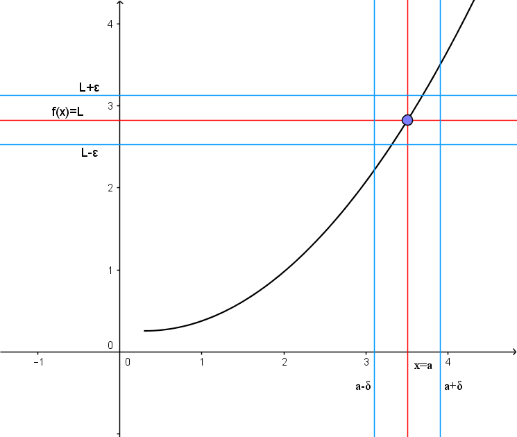
This graph represents illustration of the definition above.

1. We first pick an band around the number L on the y–axis.
2. Then we determine a ? band around the number a on the x–axis so that for all x-values (excluding x=a ) inside the ? band, the corresponding y–values lie inside the ? band.

In other words, we first pick a prescribed closeness (?) to L . Then we get close enough (?) to a so that all the corresponding y–values fall inside the  band. If a ?  > 0  can be found for each value of ? > 0, then we have proven that L is the correct limit. If there is a single ? > 0  for which this process fails, then the limit L has been incorrectly computed, or the limit does not exist.

Still not clear enough? Don’t worry, it gets better.

Intuitive definition

Let’s take a look at this function:

[latex  latex size=”2″]f(x) = \frac{(x^2-1)}{x-1}[/latex]

What is the value of this function if x=1 ?

[latex  latex size=”2″]f(1) = \frac{(1^2-1)}{1-1}[/latex]

[latex  latex size=”2″]f(1) = \frac{0}{0}[/latex]

So here we got the indeterminate. In other words, we can’t evaluate f(1) because 0 divided by 0 is not a defined value. What we can do is take a look at what happens if we approach input x=1 closely.

For example, for x = 0.5 we have:

[latex  latex size=”2″]f(0.5) = \frac{(0.5^2-1)}{0.5-1}[/latex]

[latex  latex size=”2″]f(0.5) = 1.5[/latex]

If we approach x=1 closer and closer and evaluate we get these results:

Let’s study the results from the table.

As x gets closer to value 1 (x approaches 1), the evaluation of a function gets closer to value 2 (f(x) approaches 2). What this tells us is that, although we couldn’t evaluate f(x) for x=1, we can assume it is going to be 2 but this is not mathematically correct answer.

So, what do we do?

Here’s where the limit of a function comes in handy. Using limit, we can say that the limit of f(x), as x approaches 1, is 2. This gives us a more intuitive definition of a limit.

Testing sides, left-hand and right-hand limits

Functions can be defined in many ways. Some functions have weird graphs where value y jumps from one point to another. Take a look at these two graphs for example:

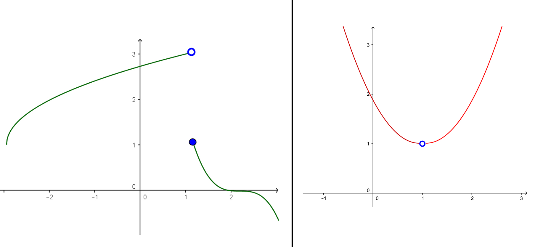
In the left graph, when input x approaches x=1 from the left side then the value of function approaches 3. We write this as

[latex  latex size=”2″]\lim \limits_{x \to 1-} f(x) = 3[/latex]

Notice that in the index we have that small ‘-‘ (minus) sign. This is how we tell that it’s the left-hand limit (approaching from the left side). For the right-hand limit it will be the plus (+) in the index. So let’s see what happens in this same graph when x approaches x=1 from the right side. We see that value of a function approaches 1, which means that

[latex  latex size=”2″]\lim \limits_{x \to 1+} f(x) = 1[/latex]

So the right-hand limit is 1. We see that left-hand limit and right-hand limit are not the same. When this is the case, the limit of function is not defined, or:

[latex  latex size=”2″]\lim \limits_{x \to 1} f(x) = \text{undefined}[/latex]

Now let’s take a look at the other graph (the one on the right).

In this graph, as input x approaches x=1 from the left side the value of a function f(x) approaches 1, so the left-hand limit is 1. When x approaches x=1 from the right side the function f(x) again approaches 1, so the right-hand limit is also 1. When left-hand limit and right-hand limit are the same then we say that ‘normal’ limit (or just limit) of the function is that value. So in our case limit of a function is 1, or:

Since:

[latex  latex size=”2″]\lim \limits_{x \to 1-} f(x) = 1[/latex]

And:

[latex  latex size=”2″]\lim \limits_{x \to 1+} f(x) = 1[/latex]

Then:

[latex  latex size=”2″]\lim \limits_{x \to 1} f(x) = 1[/latex]

What you need to remember is:

To infinity and beyond…

When dealing with limits we often need to deal with infinite valules. There are two cases. First, what happens when input x approaches infinity. The second is what happens when f(x) approaches infinity.

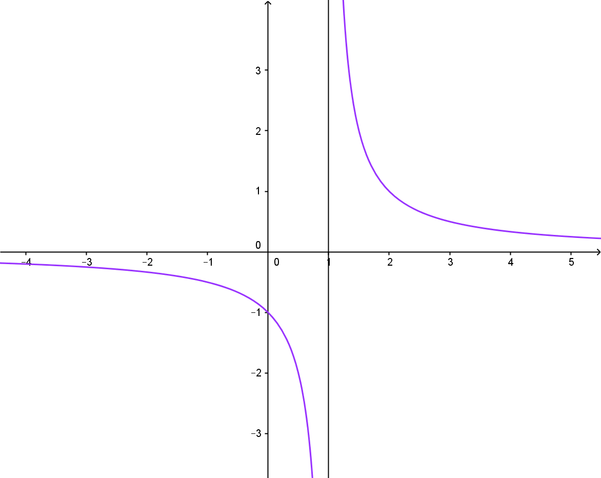
Take a look at this function:

[latex  latex size=”2″]f(x)=\frac{1}{x-1}[/latex]

Let’s approach x=1 from both sides:

[latex  latex size=”2″]\lim \limits_{x \to 1-} \frac{1}{x-1} = \frac{1}{0-} = – \infty[/latex]

[latex  latex size=”2″]\lim \limits_{x \to 1+} \frac{1}{x-1} = \frac{1}{0+} = + \infty[/latex]

We see that when we approach x=1 from left side the value of f(x) gets infinitely small (negative infinity), and if we approach from the right side the value of f(x) gets infinitely large (positive infinity). This helps us graph the function:

1. First draw a vertical line through x=1 (this is called vertical asymptote).
2. Then, sketch a function such that it approaches that line but never touches it. When approaching from the left go down (-?), and when approaching from the right go up (+?)

Now we need to examine what happens when x approaches infinity (x ? ±?). To do this we need to know this simple rule:

[latex  latex size=”2″ color=ff0000 ]\lim \limits_{x \to \infty} \frac{k}{x} = 0[/latex]

This rule is true for any real value k. Let’s get back to the example and using this rule investigate what happens when x approaches infinity values.

[latex  latex size=”2″]\lim \limits_{x \to \infty+} \frac{1}{x-1} =\frac{1}{\infty+} = 0[/latex]

[latex  latex size=”2″]\lim \limits_{x \to \infty-} \frac{1}{x-1} =\frac{1}{\infty-} = 0[/latex]

This also helps us sketch the graph:

1. First draw a horizontal line at y=0 (which is the same as x-axis and this is called horizontal asymptote).
2. Then, sketch our function such that when x ? +? (goes as far right as possible) the function approaches x-axis. Do the same thing on the left side.

Here is the graph:

Got it? Great! So next time you see a graph of a function try and think about what happens when x approaches infinity values. How do we use limits to determine that behaviour? What if f(x) approaches infinity values? This type of thinking helps you get a better feel for limits and better understanding of them.

Methods to evaluate limits

There are four basic methods to evaluate limits.

#1. Substitute x with the value it approaches.

This is the simplest method but it is rarely applicable. Here’s an example:

[latex  latex size=”2″]\lim \limits_{x \to 6} \frac{1}{x-3} = \frac{1}{6-3} = \frac{1}{3}[/latex]

Simple right? But the problem is that using this method you often get indeterminate such as 0/0.

#2. Factoring.

Consider this example

[latex  latex size=”2″]\lim \limits_{x \to 1} \frac{x^2 -2x + 1}{x-1} [/latex]

If we just put 1 instead of x we get 0/0. So we try factoring the numerator to get:

[latex  latex size=”2″]\lim \limits_{x \to 1} \frac{(x-1)(x-1)}{(x-1)} = \lim \limits_{x \to 1} x-1[/latex]

Now we just put the value in to get:

[latex  latex size=”2″]\lim \limits_{x \to 1} x -1 = 1 – 1 =0[/latex]

So the limit is 0.

#3. Multiplying by conjugate.

The conjugate of expression is the same expression except the sign in the middle is changed, for example conjugate of a+b is a-b. This method often helps when we have fractions with radicals:

[latex  latex size=”2″]\lim \limits_{x \to 4} \frac{2-\sqrt{x}}{4-x}[/latex]

Multiply both sides of the fraction by conjugate of numerator:

[latex  latex size=”2″]\lim \limits_{x \to 4} \frac{2-\sqrt{x}}{4-x} \times \frac{2+\sqrt{x}}{2+\sqrt{x}}[/latex]

Now use difference of squares formula which is a² – b² = (a – b) (a + b) to simplify the numerator:

[latex  latex size=”2″]\lim \limits_{x \to 4} \frac{4-x}{(4-x)(2+\sqrt{x})} = \lim \limits_{x \to 4}\frac{1}{2+\sqrt{x}}[/latex]

Put in the value x=4:

[latex  latex size=”2″]\lim \limits_{x \to 4} \frac{4-x}{(4-x)(2+\sqrt{x})} = \frac{1}{2+\sqrt{x}} = \frac{1}{4}[/latex]

#4 Degree of a rational function.

Rational function is of form

[latex  latex size=”2″]f(x) = \frac{P(x)}{Q(x)}[/latex]

By finding out the degree of a function we can easily determine if limit is 0,+?,-? . Example:

[latex  latex size=”2″]\lim \limits_{x \to \infty} \frac{x^3}{x-1}[/latex]

Divide both sides of the fraction by largest degree of x:

[latex  latex size=”2″]\lim \limits_{x \to \infty} \frac{\frac{x^3}{x^3}}{\frac{x}{x^3}-\frac{1}{x^3}}[/latex]

Now in the numerator we have 1 (when canceled out) and in the denominator, if we let x approach infinity, we get 1/? – 1/? = 0 – 0 = 0. So what we have in the end is 1/0 and that is +?, which is our limit.

[box type=”success” align=”” class=”” width=””]For more examples check out some of the lessons in our AP Calculus AB course. We cover everything from Limits of a Function to Areas Between Curves.[/box]