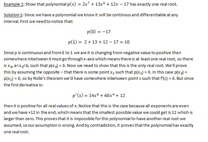
The Mean Value Theorem and its’ special case Rolle’s Theorem are two of the fundamental theorems in differential calculus. These theorems are usually learned at schools right after the derivatives and sometimes after the extreme values. They both have very clear physical and geometrical interpretations. This is why you’ll often come across problems which are based on these theorems. Aside from ‘standard’ math problems, these theorems are often required to solve ‘theoretical’ problems which aren’t so rare in tests and those types of problems are usually the ones that students hate the most. They are widely considered difficult and boring which means it is essential to understand these theorems. But don’t be fooled – there are also some very interesting problems involving these theorems and we’ll cover those too. Here, we’ll start with Rolle’s Theorem. You might wonder why we would do something like that since it is a special case of The Mean Value Theorem, but we do it because it’s the simplest special case – and also because it helps understanding  our main theorem. So without further a do, here it is:

Let’s see what this means in plain English. If you remember our lesson about extreme values (link placeholder) we said that they appear at points where the first derivative is zero. This also means that the tangent line of the function at that point is horizontal – parallel to x-axis. Knowing this, the theorem simply tells us that if the function has the same value on both ends of the interval then there must be a point inside interval at which the function takes turn – there must be some local extreme value inside. Let’s take a look at geometrical interpretation:

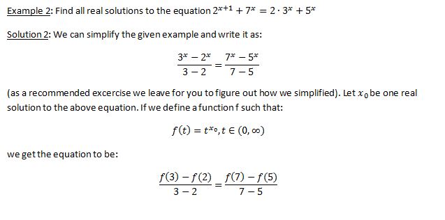
So the geometrical interpretation of Rolle’s theorem is this: if we observe two points of some contionous and differentiable (you can tell that it’s differentiable if it is smooth – no spikes) curve at which the function has the same value, then there must be some point inbetween at which the tangent line is horizontal – the first derivative is zero. Physicaly, the example of interpretation is a ball being tossed up in the air. Based on the theorem (and it’s very logical too), there will be some point in time at which the ball’s speed will be zero. This of course will happen at the ball’s highest point – the extreme value. This example’s intepretation is understandable from the graph if you look at x-axis as representation of time, and the curve is behaviour of the ball at different points in time. At point A, the ball is tossed and at point B the ball comes back down on the ground. In between, at some point it reaches maximum height – that’s when its’ speed is zero.

So after some simple factoring we got two solutions. However, we need our point c to be inside given interval, which means that the only solution will be x=2. That’s the point at which this functions’ tangent is horizontal.

Lagrange’s Mean Value Theorem

Or often just called The Mean Value Theorem can be viewed as a more general version of Rolle’s Theorem, since this one doesn’t require the function to have equal values at endpoints of interval. Here’s what it has to say:

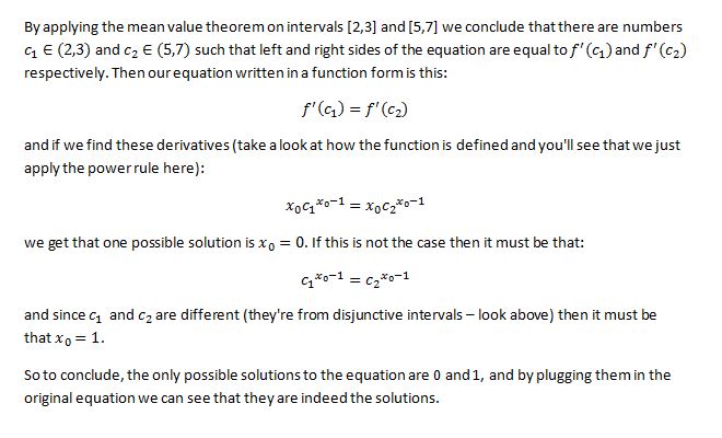
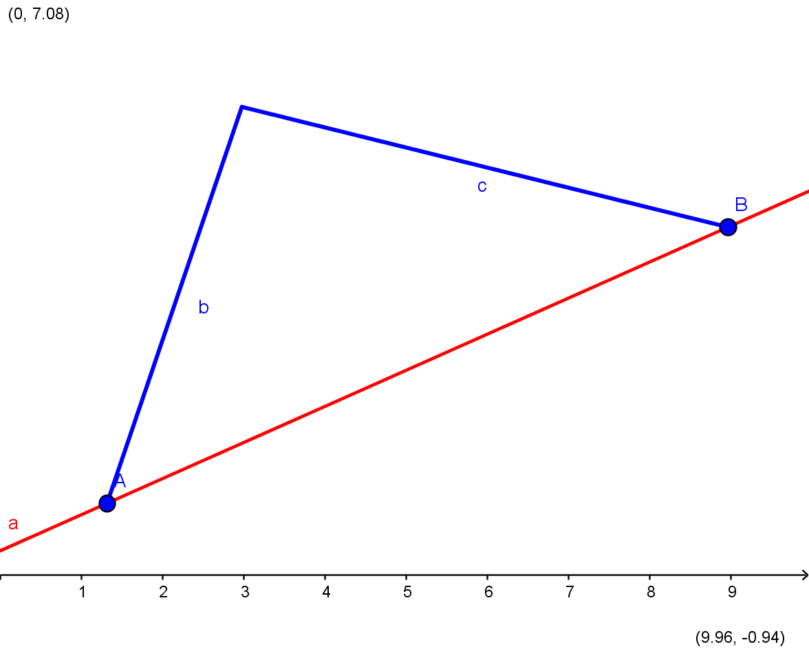
Let’s slowly go through the theorem in order to understand it. So we have two endpoints, a and b. What would be the slope of a straight line passing through these two points? The slope of the line is a change in  y divided by change in x, and in our case change in y is the difference between values of a function at endpoints f(b)-f(a) and change in x is difference between those endpoints, b – a. So the slope is . Since point c is between a and b, then the theorem tells us that for every continuos and differentiable function there is that point through which the tangent line of a function has the same slope as the slope of a secant line through endpoints. Here’s how it looks on a graph:

So geometricaly, the mean value theorem says that for a continous and differentiable (smooth) curve we can always find some point c, between two points a and b, such that the slope of a tangent line at that point is the same as the slope of a secant line through the endpoints. Physical interpretation would be something like this. Imagine we were driving from City A to City B which are 145 miles appart, and we got from one city to another in one hour. The mean value theorem says that if that is the case, then at some point in time during our journey we were driving at exactly 145 miles per hour (and greatly exceeding speed limit by doing so). In the graph, the distance between our two cities is the distance between points A and B, and the blue line would represent our speed at different points in time if we were driving at a constant speed of 145 miles per hour. Since we weren’t driving at constant speed, then our speed is represented by the curve,  and at point c we were indeed driving at exactly 145 miles per hour.

To better understand the theorem it is important to know why our assumtions are that a function is continous and differentiable at given interval. Here are two examples at what could happen if our function weren’t continous or differentiable:

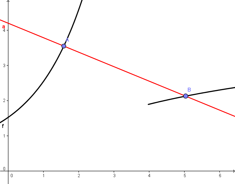
On the left side we have a function that is not contionous at (a,b), and as you can see there is no point inbetween at which the slope of the tangent line would be the same as the slope of the line passing through A and B. On the right side we have a function that is not differentiable on (a,b) (it has a spike, it’s not smooth), and therefore we also can’t find such point c.

Examples